After a three week hiatus from our safe withdrawal rate research, welcome back to the next installment! If you liked our work so far make sure you head over to SSRN (Social Science Research Network) and download a pdf version. It’s a free 47-page (!) pdf working paper covering parts 1 through 8:
But let’s move on to part 11. In our previous posts (Part 9 and Part 10), we wrote about the Guyton-Klinger dynamic withdrawal rule and why we’re not great fans. Add to that our two-month-long bashing of the static 4% rule and people may wonder:
What withdrawal rule do we like?
True, we proposed a lower initial withdrawal rate (3.25-3.50% depending on future Social Security income), but that’s just the starting point. We have written here and elsewhere that this withdrawal rate is not set in stone. How do we go about adjusting the withdrawals in the future? How did different dynamic withdrawal rules perform in the past? How do we even measure how much we like a withdrawal rate rule? Today, we like to take a step back and gather a list of criteria by which we like to evaluate different (dynamic) withdrawal rules. Then simulate a bunch of withdrawal rules and assign grades.
Withdrawal rate rules we consider
- The Fixed 4% rule: Set the initial withdrawal amount to 4% of the portfolio and then adjust by the CPI every month.
- Guyton-Klinger with a 4% initial rate. +/-20% guardrails and 10% adjustments. For a primer on what this rule does and some of the skeletons in the closet, check our previous posts on that topic, Part 9.
- The same Guyton-Klinger rule but with a 5% initial rate.
- Constant percentage: withdraw a fixed 4% p.a. of the portfolio over time (i.e., 0.333% each month).
- The Variable Percentage Withdrawal (VPW) rule, see the Bogleheads link on this, assuming a 40-year retiree (mid-point between Mr. and Mrs. ERN’s age at our planned retirement date). The same mechanics as the constant percentage, though we start at 4.6% and increase the rates based on the remaining life expectancy, calculated by smart folks at Bogleheads. In our simulations we cap the withdrawal rates at 8%, though, to ensure we don’t deplete the principal in year 60. We still like to leave a nice size bequest.
- A rule based on the Shiller CAPE: Calculate the Cyclically-Adjusted Earnings Yield (=1/CAPE) and use this as a proxy for expected equity returns. Then set the withdrawal rate to W = a + b*CAEY with the appropriate parameters for a and b. The first time I encountered this rule was at the cFIREsim site where they use this exact parameterization as their default values: a=1% and b=0.5. (There is some science behind the parameter choice and we will deal with the details in a later post!)
- Same as 6 but with a=1.5%, i.e., shift up the withdrawal rate in 6 by another 0.50% p.a.
- Same as 7 but with a=2.0%.
Here are our criteria to grade the different withdrawal rules:
- Respond to changing fundamentals in financial markets and the economy
- Provide guidance on the appropriate initial withdrawal rate
- Withdrawal amounts should display low short-term volatility.
- Withdrawal amounts don’t suffer significant and long-lasting drawdowns.
- Withdrawals have the potential to maintain purchasing power over at least 30 years
- The initial withdrawal amount is not unnecessarily low.
We will elaborate more below. For now, they should appear pretty intuitive, albeit a bit subjective. For example “low short-term volatility” means different things to different people. We will grade those criteria on a scale A = best, F = worst.
Simulation assumptions
- 80% equity, 20% bond share (S&P500 total return and 10-Year U.S. Treasury Benchmark Bond total return).
- 60 years horizon, with actual returns Jan 1957 – Dec 2016.
- Monthly simulations.
Simulation Results

Apparently, 1957 wasn’t such a bad year to start retirement. At least the 4% rule didn’t run out of money! But also notice the bumpy road during the first 30 years with a significant reduction for most of the withdrawal rules during the 1970s. In the table below we report some more stats on the final portfolio value and the withdrawals over time. Notice that the 4% rule would have accumulated a massive portfolio, more than 4 times the initial size. And that’s adjusted for inflation! So, there was ample opportunity for adjusting the withdrawal amounts upward.

And here’s the Report Card
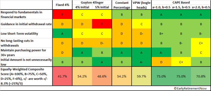
The summary of the grades we assigned here is in the table above, completely subjective and open for discussion, of course! The explanation of the grades follows.
1: Respond to fundamentals in financial markets
The top performers here are the CAPE-based rules. We set our withdrawal amounts not just based on price movements but also based on economic fundamentals (earnings yield), which earns a big fat A.
The Constant percentage and VPW both get a B because they clearly react to changes in financial conditions. If your portfolio is down by x% your withdrawal amount goes down by roughly x%, so you can’t blame it for not being responsive. But both rules lose some points for chasing price movements only and ignoring economic fundamentals (earnings!). You will overreact with the withdrawal amounts during the late 1990s equity bubble and also slash withdrawals dramatically during an equity market downturn when prices overreact on the downside.
Another notch down is Guyton-Klinger. That rule responds to changing asset prices but potentially with a delay of multiple years. You wait until you hit one of guard rails! Sorry, you get only a C for that. Of course, the static 4% rule gets an F for being completely oblivious to what’s going on in the world out there.
2: Guidance in the initial withdrawal rate
Both the fixed 4% and Constant Percentage 4% rules get a D. The 4% Guyton-Klinger Rule gets a D as well. Just picking some arbitrary percentage number is not sufficient. As we showed before in part 3 of this series, the 4% rule has very different success probabilities depending on where we are in the earnings yield cycle. The Guyton-Klinger rule with a 5% initial rate gets an F for its deceptive marketing. Sorry, but this rule cannot magically generate 1% p.a. excess return (alpha), see our posts from the last two SWR posts, here and here.
The VPW gets a C. It’s still not very good guidance given their percentage is also oblivious to market conditions, such as equity earnings yields and thus runs the risk of being too low if stocks are cheap or too high when stocks are expensive. But the effort of setting the initial withdrawal rate in response to different asset allocations and ages definitely earns the VPW a nice solid C. The CAPE-based rules get a B for at least thinking about different initial equity P/E ratio regimes. But there’s still some ambiguity about what the appropriate values for a and b should be.
3: Short-term Volatility
In retirement, we obviously have some spending flexibility, but we don’t like to go from top to flop, e.g., from a very generous travel budget in one year to a zero travel budget in the next year. We like to keep year over year withdrawal amount fluctuations to a minimum.

The simple 4% rule gets an A for having, well, zero volatility in the withdrawals. Though, when you are unlucky enough to run out of money that would be the mother of all short-term volatility, i.e., -100%. We are generous and decided to penalize the 4% rule grade in categories 4 and 5, not the short-term volatility grade, though.
Guyton-Klinger gets only a C. There is some pretty significant volatility year over year and the worst Y/Y drop is more than 25%. The CAPE-based rules have much more subdued year-over-year volatility, by construction, and get a nice, solid B; a B+ for the less aggressive rule with a=1.0% and a B- for the more aggressive rule with a=2.0%.
Both the constant percentage 4% rule and VPW get a big fat D on this one. Your withdrawal amounts become just about as volatile as your portfolio. And keep in mind that these numbers are already smoothed 12-month average withdrawals. The drawdowns peak to bottom are the same or worse as the portfolio drawdowns. To us, this seems quite undesirable. Of course, someone at the Bogelheads forum seems to claim that the VPW actually smoothes the withdrawal amounts:
“Q: Why not simply use a Constant-Percentage withdrawal instead?
A: Because VPW takes into account your current age, and allows you to eat more and more into your capital, as you age, while trying to smooth out the withdrawals.”
Though the first two claims (taking into account the age and generating an orderly exhaustion of capital all the way to age 100) are true, the VPW doesn’t do much smoothing at all. It’s just as volatile and even slightly more volatile than the Constant-Percentage Rule, and hence gets penalized another notch to a D-! The VPW percentage withdrawals increase over time and, true, if you’re lucky and increase the age-dependent withdrawal rate in a year with negative returns you would cushion the drop a little bit. But if you increase the VPW value in a year with positive returns you’d exacerbate the volatility. Most of the variance in withdrawal amounts still comes from the portfolio returns and, for all practical purposes, this method generates highly volatile withdrawal amounts.
4: No significant drawdowns in withdrawals
This was our pet peeve with Guyton-Klinger. We don’t like a multi-year or even multi-decade reduction in our standard of living. It’s easy to smooth out yearly fluctuations with some smart budgeting and a side gig here and there. But significantly reducing spending for 10-20 years means going back to work. Something we like to avoid.

Well, the 4% rule never has a drawdown until it runs out of money. As we showed in previous posts, the risk of running out of money is a serious concern when targeting 50 or 60-year horizons and considering today’s lofty equity valuations. Only a D grade here. Even though the 1957 starting date saw a great success of the 4% rule!
Guyton-Klinger, the Constant 4% and VPW all get a D on this one. The 5% Guyton Klinger even a D-. Some of the stats like the drawdown peak to bottom are truly scary.
Finally, we were very positively surprised about how smooth the CAPE-based withdrawal amounts were. The drop in withdrawals also lasts long, but it is a lot more shallow than for the other rules. Example: The intermediate rule starts at 4.5 in 1957, goes to a bit over 5.0 during the first decade, drops to 3.6 during the late 1970s and 1980s and then recovers again. During the volatile years since 2000, the declines in the withdrawal amounts were also shallow and short-term in contrast to the other rules. Good job, CAPE! We assign a B, B- and C+ for the three CAPE-based rules.
5: Maintain purchasing power after 30+ years
This one has a similar flavor as item #4 but it still a slightly different animal. We want to avoid a slow and permanent erosion of purchasing power, see illustration below:

The 4% rule has a 2.5% probability of running out of money after 30 years (80% stocks, 20% bonds), but a 37.2% probability of not maintaining 100% of its purchasing power. That doesn’t get you more a D grade in our household, and that’s when we feel generous.
Guyton-Klinger definitely does much better. True, it suffers from potentially year-long, even decade-long drawdowns in withdrawals, but after 30+ years you’re likely back to the initial net worth and the initial withdrawal amounts. In fact, if anything, you might withdraw too little and over-accumulate because the withdrawal rate is likely to be stuck at the lower guardrail. GK gets a nice solid A for the 4% initial rate and a B when starting with a 5% rule.
The constant percentage 4% rule rate gets an A because over the very long haul the expected real return of your 80/20 portfolio is higher than 4%. VPW gets an A as well. It’s obviously designed to exhaust the capital but the withdrawal amounts definitely have an upward moving trend.
The CAPE rules get grades between A- and C, depending on how aggressive you structure the parameters. Especially, the rule with a=2.0% might be a notch too aggressive and could create a slow erosion of real withdrawals over time.
6: The initial withdrawal is not too low
Any rule that withdraws a crazy low initial amount might ace some of the other criteria above but is still useless. All rules with 4%+ initial withdrawal rates clearly pass this criterion. The CAPE rules will likely fall below that 4% withdrawal rate most of the time. They had pretty competitive initial withdrawal rates back in 1957, but today, we’d be looking at only 2.7% when using the most conservative parameters (a=0.01,b=0.50) to 3.7% with the more aggressive parameters (a=0.02, b=0.50). That’s quite unattractive. But intriguingly, the one with parameter a=1.5% generates an initial withdrawal rate almost exactly at the 3.25% we proposed earlier in Part 3, and its overall grade is the highest (tie with a=1.0%). So, this might be something we will apply in our own withdrawal strategy!
Conclusion
Today’s case study taught us a lot. For a change, we intentionally didn’t look at a worst-case retirement date. 1957 was a pretty decent starting date that would have preserved the purchasing power of the classic 4% rule. But the path was rocky! The recession in the 1970s, the dot-com bust, and the Global Financial Crisis would have caused some crazy swings in the withdrawal amounts of the dynamic rules.
The Guyton-Klinger rules, Constant Percentage 4% and VPW all beat the Fixed 4% Rule. The CAPE-based rules perform a lot better at least according to our subjective grading scheme. They may afford a slightly lower initial withdrawal amount but the lower volatility going forward might be worth that cost.
Thanks for stopping by today! Please leave your comments and suggestions below! Also, make sure you check out the other parts of the series, see here for a guide to the different parts so far!
Hi BigERN,
Love the site – thanks for everything you’ve done to educate us about withdrawal rates that are actually safe!
I’ve got a couple of questions for you about the CAPE rules:
1. With all the simulations you’ve run, do you prefer certain values of the parameters a & b over others?
2. Have you considered a scenario with a more aggressive CAPE based rule and a hard cap? Something like SWR = min( 3.5% , CAPE w/ a = 2.0 & b = 0.5)
Thanks in advance!
Do you mean the max of the two? Otherwise this wouldn’t be very aggressive. Quite the opposite: You’d way too conservative when equities are cheap.
Either way, I don’t like chopping off the CAPE. Remember, the wild swings in the SWR-% would cause the SWR-$-amount to be cushioned. I like low volatility in the $ values! the % values can fluctuate all they want!
Thanks for taking the time to respond. I’m most interested in your thoughts on a & b if you care to share.
My apologies, that was a terrible explanation for #2 on my part. In terms of dollars (not %s), the minimum of the two scenarios (A & B) described below.
Scenario A: Similar to the Fixed 4% rule in this post – fixed, inflation adjusted withdrawals where the initial rate is set based on guidance from CAPE. For a typical early retiree, something like 3.5% for CAPE > 30 (today’s value mentioned in my original comment), 3.75% for 20 < CAPE < 30, 4% for CAPE < 20.
Scenario B: Withdrawals based on a CAPE rule with your favorite values of a & b 🙂
The idea is that the cap set in Scenario A limits withdrawals to an amount that the retiree is comfortable with and would serve to offset future drawdowns by letting any gains continue to compound. Incorporating the CAPE rule you retain some of the ability to respond to market fundamentals. Also I'd guess this would more closely mimic the behavior of most early retirees – not ramping spending up just because their portfolio went up, but they would potentially cut back some if the market tanks.
If you were to retire right before a crash it probably wouldn't help much, but it seems to me you'd have less $ volatility in most cases.
Please don't take this as a request to go do a ton of work and run a bunch of simulations, just curious if you've done anything like this already and I missed it on your site.
OK, gotcha. It would mean that during good times you’d never walk up your withdrawals more than CPI and save the excess for rainy days. That’s certainly a good solution. I like it! I’ve not done any simulations but intuitively this looks like a good solution. It won’t help if you retire right at the peak, but if you were to retire, say, a year before the peak you might be able to smooth your ride a little bit. Nice idea!
Wonderful post ERN. I keep referencing back to your entire SWR series and this particular post to keep myself grounded as I learn about other withdrawal rate strategies. One question on CAPE…..how would one apply a fixed income not generated from the portfolio (i.e. pension) to the overall equation in determining the amount that can be spent that year? For example, let’s say one follows CAPE and uses a=1.0 and b=0.5 with CAPE=25. The equation would result in 3% (0.01+0.5*(1/25)). If this person had a $1MM portfolio on Jan 1st and could expect $10,000 in fixed income that year that does not come from the portfolio, would the annual spending be $30,000 (3% of $1MM) or $40,000 (3% of $1MM + $10,000)? Asked another way, is any non-portfolio income over and above the spending amount calculated by the CAPE equation? As always, thanks for the help.
Great question!
I assumed that the CAPE-based formula is for the entire stock+bond portfolio, provided that there’s a large enouth stock share (60-80%).
I also played around trying to take into account both the CAPE and the bond yield. It turns out that it wasn’t worth the extra complexity.
In the “SIMULATION RESULTS” chart, can you explain how “CAPE a=1.0, b=0.5” can be HIGHER than “CAPE a=2.0, b=0.5” in every year since 1975? Assuming both equations use the same CAEY, then a=2.0 should always chart higher than when a=1.0. Thanks.
The CAPE with a=2.0 withdrew MORE during the early years than the a=1.0 version. This depleted the portfolio more and thus one has to withdraw less after 1975.
This is the big problem with “flexibility” because what looks better early on will bite you in the butt later. It’s like squeezing a balloon. 🙂
Appreciate the work, very educational, love it.
I am a little uncertain of the actual logistics.
I understand the initial withdrawal rate for the CAPE based scenarios. However, I am uncertain about the calculation of subsequent withdrawal rates.
So the next month, after you recalculated a withdrawal percentage, did you apply that to your initial portfolio value or against your remaining value?
If you always multiplied your withdrawal rate by your remaining portfolio, then you would never run out of money.
Please help us Aggies understand the mechanics of your process.
You keep computing the withdrawal rates (in %) and multiply by the remaining portfolio at that time.
Also: if you do this, correct, you will never run out of money, but you might slowly erode your purchasing power. Take the extreme case where you set the WR to 20% every year. Yeah, you never hit zero but you’ll get close to zero really quickly! 🙂
Hi ERN, do you have any thoughts on moving to equities indices that offer better value when the CAPE gets too high? For instance rather than accumulating VTI when we expect futire expected returns will be low, ie CAPE>20, instead get more non US equities with lower CAPE. I know there’s no free lunch, but it seems better to acquire at earnings yield of 5% than 4%?
I am struggling with that idea, too. On the one hand, Europe and Asia-Pacific and also EM have better valuations, measured by the CAPE. But growth sucks, especially in Europe, so this could be a cheap for a reason kind of deal.
Also, as I wrote in a post last year, the next recession and bear market will clobber every stock market everywhere again. As in every bear market before:
https://earlyretirementnow.com/2017/08/23/how-useful-is-international-diversification/
But maybe the recovery will be better abroad. Maybe wait until the bottom of the next bear market and then switch some of my stocks?
Maybe they’re cheaper for a reason as you say. Markets are efficient… until they’re not,
My struggle is that FX makes everything very complex – even though EU was cheap, the USD strength negated gains. Own (EM) stock market where I am is a case in point, local currency has done well, but in USD is at 0. Who knows what the future holds from a FX point of view. Tricky as I’m not spending in USD although USD is my benchmark because I’m located in a weaker EM currency market.
On the valuation aspect, CAPE and efficient markets, we still chase value/yield, because I cannot bring myself to buy negative yield bonds in Europe, but will acquire US treasuries. This is a case where the lowest yield is not the safest as opposed to chasing yield in the general sense.
Similarly, would I buy US equities if they were to ever go to a CAPE of 30+ but EM/EU is at single digits? My money must go somewhere, so the risk-reward looks better for lower valuation countries, even if USD strength negates some of the return in the short term.
The FX issue is important. In some of the past examples here you had very differential performance US vs. non-US, a lot of it was due to FX movements.
If you want to branch out into non-US, I’d do so gradually. Have some today already and then move more into non-US if a CAPE >30 vs. <10 ever were to materialize.
Thanks for this interesting analysis, it is definitely prompting me to do more thinking about a CAPE-based approach. I do have a question about one small piece of your post. You write
“The 4% rule has a 2.5% probability of running out of money after 30 years (80% stocks, 20% bonds), but a 37.2% probability of not maintaining 100% of its purchasing power.”
Given that the fixed 4% rule assumes a CPI adjustment each month, where (aside from the possibility of running out of money) is the probability of not maintaining purchasing power coming from? I would have naively assumed that the CPI adjustment basically guarantees that purchasing power is maintained while there’s money left. What do the 37.2% of scenarios where purchasing power is not maintained look like? Thanks again.
37.2% of the time your final portfolio value was below the initial portfolio adjusted for inflation. 2.7% of the time the final portfolio value would have been below zero, i.e., you ran out of money before the 30Y mark.
Ah, my confusion was reading “Withdrawals have the potential to maintain purchasing power over at least 30 years” as referring to the purchasing power of the withdrawals themselves vs. the purchasing power of the overall portfolio. I’d assume that this is criteria is more or less relevant depending on overall timeline and individual preference for having funds left at “the end”. Thanks for the quick response!
Yeah, took me a while to figure this one out, but I finally did. This refers to the “final” value after 30 years. Pretty positive that the grade is in the context of an early retiree planning for 50-60 years of retirement. But ERN does most of his analyses with 30 year time periods, because you can miss to much when only looking at 60 year periods. So you consider two 30 year periods, but for it to work you need to retain most (80%+?) of your portfolio at the end of the first 30 years to be able to make it through the second 30.
For a traditional retiree, seems to me this row would go away entirely (the static 4% rule gets dinged in the row above, though maybe you changed the D to an F)
I’m thinking on a very simple dynamic withdrawal rate method that seems to make a lot of sense to me:
“Starting over” the fixed 4% rule whenever desirable.
That is, each year our withdrawal is max(4% of original value + inflation, 4% of current value)
(Though personally, I would prefer 3.5% rather than 4%).
This rule enables to enlarge your withdrawal in the common case you portfolio has a lot of gains (or you got some extra cash that you would like to feed into your portfolio, or did not spend all of last year’s withdrawal), but still maintain that minimum living standard on bad years.
The mathematical idea behind this is that there’s nothing special about your specific retirement year or retirement sum, and you can always say “I’m restarting my retirement!”
The downside is, of course, that you change the statistics of the retirement years (instead of retiring on a specific year, you are now “retiring” on dozens of different years, which are the better stock market years), so a lower withdrawal rate would be beneficial, like you suggest for the high CAPE retirements.
I would love to see an analysis of the SWR for this withdrawal rule.
I found a great analysis in
https://thepoorswiss.com/withdraw-current-portfolio/
but it doesn’t go all the way to a 60 year retirement.
You’d walk up the withdrawals when the market does well, but you will not walk down the withdrawals when the market does poorly.
What can possibly go wrong? At some point there will be a time when the 4% Rule fails. 1929, various times in the 1960s. Possibly 2000. Possibly 2021. By ratcheting up the withdrawals but never ratcheting down you will eventually reset the withdrawal amount to 4% at the market peak when the 4% Rule fails.
So, this approach is not only no solution to the Sequence Risk Problem. It makes the Sequence Risk problem worse.
Thanks for considering this.
I think what you say is true if the withdrawal rule was max(4% of previous year+inflation, 4% of current value).
In my suggestion, you do ratchet up but you also ratchet back down to your starting withdrawal (+inflation) when necessary.
Let’s consider a very bad case of retiring just before the big recession, say 1927 (obviously retiring at the peak at 1929 would be identical to the fixed 4% rule since the portfolio would not rise above it).
So, the withdrawal rate would be slightly higher in 1928 and 1929 since the portfolio went up, but that’s it. at 1930, the market plummets and we go back to withdrawing 4%+inflation of the original 1927. This limits the over-withdrawal to only two years, that shouldn’t have a large influence on the SWR and can easily be mitigated by taking a slightly lower withdrawal rate (or at least I think it’s interesting to see in simulation).
On the plus side, in majority of retirement scenarios, the median portfolio rises significantly above the initial retirement portfolio. I’m looking for a rule that would define how much and when I can withdraw more than the fixed 4% rule, when it is obvious that it does not pose a failure threat.
Additionally, maybe sequence risk alleviation could be done using a moving average:
withdrawal = max(4% of original value + inflation, 4% of average portfolio value in last 7 years).
This means that the “current” argument would not be activated at all on the first 7 years, and after that only on a very smooth average basis.
OK, gotcha. It’s less risky if you also ratchet down.
The median portfolio is irrelevant. Unless you find some retirees from earlier/later cohorts that are willing to help you out and give you some of their money.
We have to very few early retirement planners or bloggers question the validity of the 4% safe withdrawal rate rule. The 4% rule is a guideline used as a safe withdrawal rate, particularly in early retirement, to help prevent retirees from running out of money.
I picture the parameters “a” and “b” in Withdrawal Rule 6 as follows.
b = 0.5 is equivalent to a sustainable dividend yield that is 50% of the earnings yield. If one thinks of one’s portfolio as a mini-conglomerate of dozens to thousands of partially-owned subsidiaries, selecting a safe withdrawal rate is equivalent to setting a sustainable dividend yield for the conglomerate. To the extent subsidiaries are held in mutual funds, the average expense ratio of the funds should probably be subtracted from the earnings yield before multiplying by b.
The parameter “a” is clearly related to growth, but growth rate of what? Perhaps for the S&P 500, the real US GDP is a logical growth rate for comparison? Historically, the trailing 25-year average US GDP has dropped from around 4% in the early 1970s to about 2.5% by the late 2010s. Multiplying these values by b=0.5 gives an estimated range of a from 2% (early 70s) to 1.25% (late 10s). If the real US GDP sets the scale for the parameter “a”, perhaps one should avoid using a > 1%, and keep an eye on whether the GDP continues to drop with time?
We can interpret the parameters all sorts of ways.
The CAPE yield is related to the real growth of the portfolio. Not really GDP (though the two are related).
If you set b=1 you’re back at a regular fixes WR, because the rate exactly ofsets your portfolio gains/losses and keeps the amount roughly constant.
If you set b=0 you are back to the constant percentage rate equal to a.
At b=0.5 you are half-way in between.