
Welcome back to the Safe Withdrawal Rate series. 13 installments already! As requested by many readers, both in the comments section and via email, I wanted to look into one intriguing method, called “Prime Harvesting” (PH) to dynamically shift the stock vs. bond allocation during retirement. Where does this post fit into the big picture? Recall that parts 1-8 of our series dealt with fixed withdrawals and fixed asset allocation (same % stocks and bonds throughout retirement). Make sure you check out our SSRN working paper, now downloaded over 1,000 times!
Parts 9-11 dealt with how to adjust the withdrawal amounts while keeping the asset allocation fixed (Guyton-Klinger, VPW, CAPE-based rules, etc.). Prime Harvesting does something completely different: Keep the withdrawal amount constant, but use a dynamic stock/bond asset allocation to (hopefully) squeeze out some extra withdrawal wiggle room; the Northwest corner in the diagram below. Almost uncharted territory in our series!

Eventually, of course, we like to move to that Northeast corner: Dynamic withdrawals and Dynamic Asset Allocation. But let’s take it one step at a time! Let’s see what this Prime Harvesting is all about.
Let’s get cranking!
Basic McClung Prime Harvesting Rules
- This rule was proposed by Michael McClung in his book Living Off Your Money (paid link).
- Pick an initial asset allocation, e.g., 60% Stocks, 40% Bonds.
- There is an upper “guardrail” for the stock portfolio. You never withdraw from the stock portfolio until you reach that upper guardrail of equity holdings (and the guardrail is adjusted for CPI inflation). Normally that guardrail is set to 1.2 times the original equity holdings.
- If stocks are at or above 1.2-times their initial level (adjusted for inflation) then sell 20% of stocks and shift into bonds.
- Sell from bonds to fund upcoming withdrawal. If no more bonds are available then sell stocks.
- That’s it. It’s really that easy!
Why this works
Prime Harvesting has the tendency to first liquidate bonds and let equity gains run for a while before withdrawing. If you have the bad luck of an equity drawdown early during retirement (sequence of return risk!) you avoid selling stocks at the bottom and first live off the bond portfolio until equities recover. Smart move!
You could potentially get lower sustainable withdrawal rates if equities have a very long and sustained bull market (1991-2000) and you start liquidating equities too early by consistently breaching the upper guardrail. But that’s when you least worry about suffering a slightly smaller safe withdrawal rate: 7% or 8%, who cares? PH helps you when you need it the most: when the fixed withdrawal method only sustains a sub-4% withdrawal rate. Of course, the idea isn’t new. Wade Pfau and Kitces have a paper on this exact topic: Why you want a rising (!) equity glide path in retirement. I wrote about the idea of rising glidepaths in Part 19 and Part 20 of this series.
Here are a few things that we don’t like about this approach:
- The analysis is done annually in the McClung book. We don’t like to withdraw an entire year’s worth of living expenses all at once, so we want our simulations to run monthly rather than annually. The simulations also have to be consistent and comparable with our other simulations!
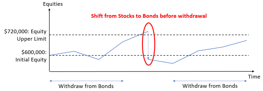
- The equity rebalancing rule in its proposed form sounds a bit nonsensical. Imagine you start with a million dollar portfolio, $600k in stocks, $400k in bonds. The upper limit for stocks is $720k. Imagine you’re at $719,999. You do nothing. Just one additional dollar and you’d sell a huge pile of $144k worth of stocks and bring the equity holdings to below (!) the initial level. That seems a bit excessive. I found that a more sensible way would be to shift down to $600k (=> reduce by 20% of the original equity weight). Maybe the explanation in the book wasn’t entirely clear and this is what McClung meant. Whatever his intention, this is what I use as the McClung rule.
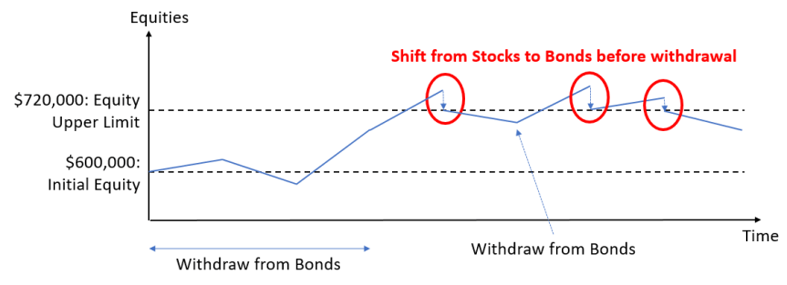
- Even that modified McClung rule creates some pretty nonsensical outcomes, more details below. Instead of selling a lot of equities all at once after breaching the upper guardrail, I also propose a new version, McClung-Smooth, where we sell only enough equities to bring the equity holdings back to the upper guardrail.
Let’s see how the PH methodology would have performed when applied to some of the “trouble-maker” retirement cohorts.
Case Study: 1966
- Monthly Simulations: January 1966 – December 1995 (360 months)
- Pick one initial withdrawal rate (in % of initial portfolio), and adjust the withdrawal amounts by the CPI index regardless of portfolio performance.
- Initial portfolio: 60% stocks, 40% bonds.
- Target capital preservation, so the final portfolio value is the same as the initial, adjusted for inflation after 30 years. Recall that my wife, Mrs. ERN, will be 64 after 30 years of early retirement so I would prefer to preserve capital for at least 30 years.
- The guardrail is 1.2 times the initial value, adjusted for inflation every month.
The asset allocation rules we consider:
- McClung: after breaching the upper guardrail, sell 20% worth of equities of the original, inflation-adjusted equity holdings, e.g., with a $1,000,000 portfolio shift $120,000 (adjusted for inflation) of the equity portfolio into bonds.
- McClung-smooth: after breaching the upper guardrail sell enough stocks to bring the equity holdings back to the guardrail.
- Forced bond liquidation: Same as above, but with an infinite equity guardrail. This has the effect of never shifting from stocks to bonds, i.e., we live off the bond portfolio (principal + interest) until bonds are exhausted and then just maintain a 100% stock portfolio.
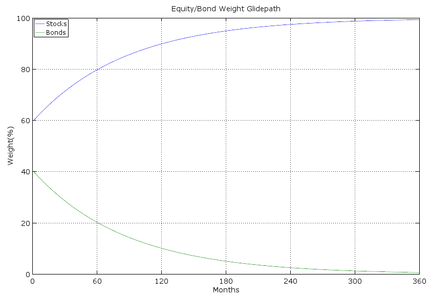
- Glidepath: We shift to a to a 100% stock, 0% bond portfolio. From a 60/40 portfolio, we steadily converge to a 100/0 portfolio.
- Fixed: We keep a fixed 60/40 allocation.
Results:
First, let’s look at the maximum sustainable withdrawal rates that guarantee capital preservation:
- McClung: 3.038%
- McClung-Smooth: 3.071%
- Forced Bond Liquidation: 3.069%
- Glide Path: 3.061%
- Fixed Withdrawal Rate: 2.815%
Nice! With a rising equity glidepath, we beat the low fixed withdrawal rate. But don’t get your hopes up too high. We are talking about a 0.2% difference, $2,000 p.a. in a $1,000,000 portfolio. Not that McClung ever claimed otherwise, but the advantage of the PH method is small. But it is consistent, i.e., we never found a retirement cohort where the fixed SWR was below 4% and the PH method hurt you.
How does the McClung experience look like over time for this cohort? In the chart below we plot the time series of stock and bond levels (top chart, scaled to initial portfolio value of 1.0) and stock and bond portfolio shares as a percent of the overall portfolio. 1966 was a very challenging year. You slowly erode your bonds over about 12 years and then live off the pretty badly decimated stock portfolio. Only when equities recover in the 1980s would you start replenishing the bond portfolio in the late 1980s and early 1990. Notice the four big distinct and discrete jumps in bonds!

The smooth McClung method is exactly identical to the above chart until 1987 because it never hit the upper guardrail for two decades. The shift into bonds is a little bit more gradual. Equities hover around the 0.72 mark for most of the remaining years of the simulation horizon and all the gains above that mark are skimmed off into the bond portfolio. It’s no wonder that the smooth McClung method performs a little bit better than the original McClung method; you keep a higher average equity portfolio during the stock market heydays of the late 1980s and mid-1990s.

Yet another scenario, the forced bond liquidation never moves back into bonds in 1987. Despite the crash in October 1987, you achieve capital preservation with a withdrawal rate not too different from the smooth McClung method.

Something fishy going on with McClung?
Working on this research project, I noticed something odd. Below I plot the final value of the portfolio as a function of the withdrawal rate for both the McClung and McClung-Smooth allocation rules. Each tick mark is 0.001% (that’s only $10 annual withdrawal in a $1,000,000 portfolio). For the original McClung, the final value is non-monotone (!) in the withdrawal rate. There are several occasions where the sustainable withdrawal rate moves up (!) when you increase the withdrawal rate. But there are also cases where the final value plummets by a significant amount by merely increasing the initial withdrawal amount by one tick mark. How is that possible? It has to do with the discrete shift out of equities and into bonds as mandated by McClung.

So imagine with a 3.010% withdrawal rate we reach $719,999.99 by a certain month. With a 3.009% withdrawal rate, we’d have reached just a few dollars above $720,000. What if we shifted the $120,000 out of equities, as mandated by McClung, right before another big blockbuster month in equities? It’s possible that we might shift out of equities exactly at the wrong time and end up with a lower final value despite a lower withdrawal rate. But “Natura non facit saltus” which is why we prefer our smooth McClung version (the green line). Thus, as much as I like the spirit of the McClung procedure, the implementation as recommended in his book is unacceptable. You should not get a final value that’s not monotonically decreasing in the withdrawal rate. And, likewise, a change of 0.001% in the initial withdrawal rate making a difference of 5%+ in the final portfolio value is preposterous. This would imply that in a $1m portfolio, a change of $10 in the initial annual withdrawal amount would translate into a $50,000 difference in the final value.
Other cohorts
Let’s compare the safe withdrawal rules of other cohorts as well. January 2000 would have been another bad retirement date. To preserve the capital over the next 17 years, a fixed withdrawal amount, adjusted for CPI, would have sustained only a 2.652% initial rate. Again, the McClung-style rules would have outperformed that rate. Quite intriguingly, the glidepath performed the best. Though, the differences are all very small!
Starting retirement at the market peak in October 2007, the fixed withdrawal rate would have supported an initial SWR of just under 4%. McClung again beats this by about 0.20%, but the McClung-Smooth procedure again does better than the regular McClung. Quite intriguingly, the forced bond liquidation and the glidepath beat both of the McClung rules by a very substantial margin.

An important caveat
Let’s look at the chart of equity/bond holdings/percentages for the January 2000 retirement cohort using the McClung-smooth rule. The SWR is only 2.742%. But notice how this retiree never even touched the equity portfolio until 2014. How can a $400k bond portfolio sustain $27,420 p.a. in withdrawals for 14 years and be only half depleted by 2014? That’s a withdrawal rate of 6.855% out of the bond portfolio plus inflation adjustment! We never depleted the fixed income portfolio because bonds did phenomenally well during that period. Yields started at over 6%, then yields went down due to Fed policy (lower target rate, quantitative easing, etc.) and brought large capital gains in bonds. What are the odds we’ll have another bond bull market going forward? Slim to none. Current yields on 10-year Treasury bonds are only slightly above 2%, so average bond returns over the next 14 years can’t possibly match the return of the 2000-2014 period. So the caveat here: Prime Harvesting works best if bonds do well. But that may not be the case over the next few years!

Conclusion
Prime Harvesting is an intuitive method to dynamically shift the stock/bond allocation in retirement. In the past, it would have sustained slightly higher withdrawal rates than the fixed percentage rule when it mattered the most: when stocks did poorly right after retirement. We propose one improvement to this methodology; use a smoother version that avoids selling massive amounts of equities all at once. Letting equities rest at the upper guardrail and skimming only the excess equity wealth above the guardrail seems to be a more sensible approach. It not only avoids the discontinuities and jumps in the final asset value chart above but also tends to afford slightly higher SWRs.
In some of the simulations, we found that just a naive glidepath toward higher equity percentages beats even the more complicated McClung procedure. But that comes at a price: Do people really have the appetite for 100% equities later in retirement?
We are particularly interested in how the Prime Harvesting rule will interact with dynamic withdrawal amounts. That’s because in retirement we’d not even be very interested in increasing our withdrawals if the market does well. Instead of buying more consumption (who wants that, we’re all frugal around here, right?) we’d probably prefer to “buy more safety” by de-risking the portfolio and shifting into bonds instead. Prime Harvesting would be a good tool to achieve that. But as always, in 2,000 words or so we can only scratch the surface. We are planning more installments of this series, so check this space for more research on this topic!
Thanks for stopping by today! Please leave your comments and suggestions below! Also, make sure you check out the other parts of the series, see here for a guide to the different parts so far!
Picture source: pixabay.com
Thanks for posting this! That issue with the discontinuity is a concern but that’s a very elegant way to solve it! Great job! I was afraid you’d give McClung the “Guyton-Klinger” treatment over that one.
One other question: In the time series charts with the S/B levels it looks like the final value doesn’t add up to 1.000. It’s most visible in the bond-depletion model. Or do I see this wrong?
Thanks!
That’s right, I actually like the spirit of the McClung technique. Just tried to find a way to execute a good idea a little bit better! 🙂
About the charts:, my God, you have sharp eyes. The portfolio levels I plot here are the beginning of the month levels, after the rebalance but before the withdrawal. On Nov30/Dec1 of 1995 you ended up slightly below 1.000, but then after the withdrawal and the December return (~2.8%) you reach the 1.000 spot on. That’s how the SWR was calculated: to exactly match the end-of-the-month.
Cheers!
I’m curious how the math works out with a cash safety cushion and a much smaller bond allocation, which might better match the results of your previous studies for people getting close to retirement.
60/40 seems to belong to an era when the Feds could survive paying 4% interest on their debt…
It will be worse. I tried to replace small amounts or all of the bond portfolio with cash and you need the extra yield from bonds over cash and the negative correlation in the 2000s to get you through the tough times.
Also: What happens when we do 80/20 or 90/10. Then the McClung-cushion is too small to get you trough the recession and you do withdraw at an inopportune time.
Thanks!
Big ERN,
Oh boy! Another fantastic post! McClung made more understandable and better!!! Excellent critical analysis!!!
Too bad I couldn’t contemplate existence, the universe, the meaning of life, and your latest blog post at w*rk today. Not sure where the day went, but I think I was actually doing what I was supposed to be doing. Whaaaaat?!?!?
Anyways, your allocation/withdrawal quadrants is a beautiful summary of the landscape. Other than reigniting (hehehe–FIRE reference) the PTSD from lectures from a nonparametric statistics course in my past (the prof just loved to use a 2×2 dichotomization grid to show how he had found unexplored areas in statistics), I just cannot wait until you blow through (air) the dynamic/dynamic quadrant, wash away (water) any turbidity, and dust away (earth) any misconceptions to unleash the fourth element—FIRE!!!
McClung clearly favors EM (Extended Mortality Updating Failure Percentage) based on his explorations for a dynamic/dynamic strategy. Can’t wait to read your insights and observations.
Thanks Dr. FIRE! Always looking forward to your feedback!!! Yes, in the McClung book there’s more than Prime Harvesting. More interesting stuff to simulate in the dynamic/dynamic quadrant! The fourth element in the first quadrant! 🙂
Cheers!
I was excited to see a variable allocation post but I was hoping it would be based on valuation or trend following. This approach seems somewhat arbitrary.
We all have to start small, right! 🙂
I like the McClung rule as an asset allocation tool because it’s easy. You can follow this rule without any tools or data except your brokerage statement.
But to be sure: McClung has a flavor or valuation. You sell equities when they rally, hold on the equities when they are cheap. It’s a poor man’s version of valuation. 🙂
Thanks for the post!
There is a long thread on Bogleheads about the McClung book. On it, the primary author of VPW, longinvest, raises an objection (which by the way is also an objection to the traditional SWR notion). His post is here: https://www.bogleheads.org/forum/viewtopic.php?f=10&t=192105&start=150#p2981105.
Basically, he objects to having a memory property built into a withdrawal system that relies on the initial conditions of your retirement. In this case, the cap on equity is calibrated to your initial portfolio. I think this creates the perverse situation where two people could have identical portfolios and identical ages (i.e face the same future), but have arrived there with different histories and thus derive different recipes for withdrawal.
Anyway, food for thought . . .
This is a great comment. Thanks for pointing that out. This problem about “memory” has a name in dynamic optimization: One would say, it violates the Principle of Optimality. See here:
https://en.wikipedia.org/wiki/Bellman_equation
Especially this part:
Many withdrawal rules (SWR, Guyton-Klinger) and the McClung asset allocation rule violate this principle of optimality for exactly the reasons mentioned. On the other hand: VPW, constant percentage and CAPE-based rule satisfy this principle. In fact, if you remember our part 11 of this series, I initially had another criterion “satisfies the Principle of Optimality” but I decided to not include that because it sounded too technical.
But I once mentioned the time consistency problem here in a very early post on the SWR:
https://earlyretirementnow.com/2016/04/15/pros-and-cons-of-different-withdrawal-rate-rules/
Anyway, as much as I consider the violation of PoO a problem, McClung has a certain appeal. It’s a quick and dirty way of implementing valuation. But point well taken. Thanks for stopping by!!!
Hi ERN,
I was also thinking about this problem. The solution I have come to for my personal SWR is the following:
Withdraw the lesser of the two p.a.:
-2% of the portfolio’s all-time high for my portfolio
-4% of the current portfolio value
I am in a global all equity portfolio and I want the portfolio to continue to grow in retirement as I age.
What do you think?
Thank you,
Matt
I also wonder if my portfolio’s concept would be something that would be possible for you to model in the future:
The concept of trying to further accumulate wealth after retirement; we don’t need a high SWR now, but in 10 years or so we are thinking of potentially having children and increasing our expenses for luxury and healthcare as we age. I also wonder what you think about using the previous high as the portfolio value for the 2%SWR. It would be interesting to see what our wealth accumulation would look like as well as our progressive withdrawals overtime using this method.
Thanks again!
Matt
You can easily model the increase in future spending. There’s a feature in teh Google Sheet where you can add above/below normal cash flows.
Previous high and then 2% seems really low. You should set the SWR to the fail-safe a the previous high, which will likely be 3.25-3.5%.
But Family 2 would therefore have fewer years left in their retirement than family 1 assuming both 1 and 2 have the same total years of retirement. So Family 2’s $1m @ $50k/year is not the same as Family 1’s $1m @40k/yr.
No, I was assuming family 2 reatired x years earlier but also x years younger. When they find themselves in that same year with the same portfolio at the same age and have the same horizon: why would family 1+2 withdraw different amounts?
It’s a violation of the principle of optimality.
Big ERN,
You had me at Bellman <3!!!
Ahhhhh, the joys of dynamic programming (DP). What a beautiful set of topics to inflict trauma on graduate students!!! Lagrangians, Hamiltonians, Transversality Conditions, First Order Necessary Conditions, Second Order Conditions, State Variables, Controls, … — at the end of the semester, parting was such sweet sorrow! Alas, recalling my days in studying DP, there was a noticeable gap in what is needed for ER analysis. I only recall fixed horizon optimization and infinite horizon optimization. Unfortunately, ER demands a stochastic horizon IMHO–something in-between the Cake Eating Program and the Mushroom Grower's Problem (not 100% sure on the names of "classic" DP problems). Based on all the WR I have studied since my DP pain induction days, is it safe to assume that stochastic horizon DP problems are just really freakin' hard?!?!?! Or is there a branch of this field that I am blissfully unaware of?
Ha, a fellow Bellman equation fan! Who would have thought?!
I would model the retirement problem as a finite horizon problem. Assume everybody dies for sure at age 110. Then roll the Bellman equation backward with age as an additional state variable and stochastic survival probabilities, also dependent on age. Maybe I will tackle that one of these days if I have some quiet time on the weekend… 🙂
Seems like a reasonable approach. However, as we all should have learned from The Cruciferous Vegetable Amplification episode of The Big Bang Theory, Sheldon clearly shows that “the singularity… when man will be able to transfer his consciousness into machines, and achieve immortality” will occur in the not too distant future and completely change your proposed workaround. Case closed. Or is it case open? Or, maybe, clopen?!?i? 😉
I’d be interested to see an exploration of what happens when a retiree attempts to maintain a constant (real) dollar allocation to equities, keeping anything extra in bonds. Say 25x annual expenses in equities – if they go up in a month the extra is skimmed off into bonds, if they go down bonds are sold to purchase add’l equities. This seems similar to the approaches here except you’d be buying back into equities during a downturn.
Interesting idea! Have to see how to implement that! This obviously also relies on accumulating a little bit extra beyond the 25x, otherwise, you’re starting out with 100% equities.
Basically the idea is that at the end of every month if your portfolio value is less than N times your annual spending you rebalance to 100% equities. If it’s greater, you keep N x spending in equities and the rest in bonds. I played around with it using your google docs toolbox (thanks!) and found that it seemed to perform well and that good values for N seemed to be in the 19-25 range.
Nice! Thanks for sharing. It’s on my long to-do list. Maybe when I’m retired?! Oh, that’s next week! 🙂
I like the Prime Harvesting Smooth approach but I am curious at the guardrail decision. McClung (and you) set it at 120% of the original dollar value of equities adjusted for inflation. But that is clearly an arbitrary rise. Have you run the numbers using a lesser jump, e.g. 110%. I am curious whether a bonds first approach with a smaller equity guardrail ceiling results in similar results.
Fantastic post! I love the idea of glidepaths, forced bond liquidation, prime harvesting, etc, but a major concern I have is how taxes could hurt you while “rebalancing”. Each time you sell equities and buy bonds, there is a tax bill to pay which can significantly drag down your safe withdraw rate. Do you plan to do any analysis or research into how taxes play into these sorts of glidepaths or even just annual rebalancing in general?
Good point. One could to the glidepath by shifing the marginal S/B allocations inside the tax-deferred accounts so as to avoid any unnecessary cap gains.
Just come across this interesting set of posts, a lot of work has been done.
Having recently read the McClung book, he does advocate a 20% sale of equities to bonds at the trigger point point of a 20% real gain in the equity portfolio, ie to below the original level.
He does offer an “Alternative Prime Harvesting “ method where the portfolio is rebalanced to the original equity / bond ratio when equity reaches a real 20% gain. This tends to offer a different dynamic of the equity bond ratio throughout the life of the portfolio and finally he offers a “get out of jail free” card, if you feel the portfolio rebalance is going to be uncomfortable , then you can restart the process with a reset. Enter the new ages portfolio balances etc and off you go again.
The book is detailed and balanced and not prescriptive, there’s room to vary the details if one is feeling uncomfortable.
All good points. I adhere to the principle “natura non facit saltus” so I’m uncomfortable moving one large big chunk of the portfolio just based on a trigger. There’s too much risk of getting the timing right/wrong. But overall it’s a nice book.
ERN, I am slowly working my way through all your SWR posts in order, and this is my favorite one yet. With McClung-Smooth, I can finally begin imagining a SWR process which seems reasonable to me. I am still 5 years away from my FIRE date, but preparing now for my plan. My question is–and maybe you get to this later in the series–which SWR plan are you using, now that you’re retired? Thank you!
I Lime the CAPE-based Rule, see Part 18 for the withdrawal Rate.
I have to admit I don’t have as much bond exposure as McClung recommends as the as his starting point. But I got some other income generating assets (Put Writing, real estate) to deal with Sequence Risk.
No, McClung is very clear about the method. See the example on page 92. It’s 20% of the current amount, not the original amount.
Thanks for your careful analysis of all these approaches. After reading a few, I’ve realized your analyses don’t have much applicability for me or most people, given the extreme early age of retirement and thus the goal of 30 years of capital preservation. Even most people who are retiring early are retiring in their late 50s or early 60s. But it’s nonetheless been interesting reading through what you’ve done on the topic.
I’m only stopping now because I’ve realized it’s a tremendous waste of my time to chase false precision in a system that doesn’t have any really good dynamical rules. So much back-testing in this arena (and typically in only one country – although McClung at least looked at three), so little forward-testing that it breaks my little scientist heart. (As an astronomer, I fully understand the difficulty of forward-testing dynamically slow systems – we have processes where a billion years is “quick” – but you can at least have training sets distinct from test sets.)
I don’t know if you address this in one of your numerous posts, but I’d be interested in the effect on overall well-being of striving to achieve a good work–life balance rather than focusing on accumulating boatloads of money to retire very early. Those who are in high-earning careers and thus able to retire early also should mostly be those who have intellectually stimulating career fields. A laser focus on retirement in one’s 30s seems like a sign something is wrong in one’s career. Those who justifiably have no interest in their jobs (e.g., an Amazon warehouse employee) aren’t those able to seriously consider retirement that young.
I don’t care what McClung meant on page 92. I care about whether this rule makes sense or not. It doesn’t. Hence my comment:
But in any case, sorry, I wasted your time. I think it’s more efficient for you to look elsewhere for the topics that interest you, than for me to change my style. Best of luck!
So – what about that upper right quadrant?? Dynamic asset allocation with VPW – yes, please!!
I read McClung and loved it – at least it provided a plausible alternative strategy to simplistic fixed withdrawal rates and AA’s. This is getting very real for me, as we pull the pin on wife’s job in a few months, and I’m already out. So I need to get our decum plan dialed in better.
Still catching up on your recommended sections on VPW – thanks for those!
MCClung is operationally not very different from a Glidepath. See Parts 19-20.
I have McClung’s book but it seems too much of a datadump with limited use for me personally. I need a spreadsheet to play around with the sims.
Did you ever write the post on the 4th quadrant – prime harvesting also considering variable withdrawal rate and not just fixed? Sorry if I missed that but would be really interested to read it.
I am worried about sequence risk in the few years before retirement too, extending my career length. Considering “bond tent” 10 years prior, 10 years after (70/30 to 30/70 back to 70/30), prime harvesting the 70/30 after that, with a 5% of current portfolio / 3.5% floor withdrawal rate. In my mind this solves (as best I can) for Sequence Risk, “what to sell”, and how much to take, while not likely leaving such a huge pile at the end and not enjoying it.
We retired in May 2022, right in the teeth of the 2022 market collapse, inverted yield curve, falling bond prices and rising inflation. In other word, the SORR post child.
Fortunately my advisor had encouraged me to keep three years of living expenses in cash as a reserve (not “emergency” – a key conceptual difference) for just such an occurrence. While I certainly wasn’t expecting to have to use it from Day 1 of our quitting work and stopping the paychecks, I sure was glad we had it because we did use it and continued to use it through 2023.
It was only in January this year (2024) when I finally decided to liquidate some equity positions to harvest some cash and replenish my reserve, this time in a five year bond ladder. As those mature I’ll have an instant pile of cash available for spending or reinvesting, depending on which way the market is going.
So call it VPW with Kentucky-windage-based Prime Harvesting. Behavioral finance VPW?
Good advice. Bonds would have been bad with yields so low back then. Cash (money market, 3M T-Bills, etc.) worked really well.
See part 43: Yes, it’s best to scale down risk before retirement, then go back into stocks. Also called a bond tent.
4th quadrant as in Southeast? Yes, my posts on the CAPE-ratio-based withdrawals. See parts 18, 54.
Sorry should have stated that better – North East. Variable Asset Allocation and Variable Withdrawals.
Haven’t written anything on that quadrant yet. But it’s on my agenda to introduce some ideas for tactical asset allocation plus CAPE-based rules.