
Welcome to the newest installment of the Safe Withdrawal Series! Part 25 already, who would have thought that we make it this far?! But there’s just so much to write on this topic! Last time, in Part 24, I ran out of space and had to defer a few more flexibility myths to today’s post. And I promised to look into a few reader suggestions. So let’s do that today pick up where we left off last time…
Updates on the rules suggested by readers
People came up with two interesting suggestions I hadn’t considered before. So I wanted to feature the simulations for those as well:
- What about starting with a cash bucket, i.e., having 2-3 years worth of spending stashed away in a money market account or short-term CDs to access if the market doesn’t cooperate? Sounds a little bit like Fritz’ Bucket Strategy.
- How about we cautiously start at 3.25% and then have the flexibility to walk up our withdrawals if the portfolio grows enough over time? How long would it take to actually grow withdrawals in the cohorts where the 3.25% turned out way too low?
Notice that both rules have one thing in common: the withdrawal rate is below 4%! Let’s not even try to make the 4% Rule work because we can’t. Any new alternative flexibility scheme that may look better than the existing ones in year X has to sacrifice something in another year Y. But obviously, we can get somewhere if we consider the flexibility of simply working another year or two and adding a cash cushion or a lower SWR. Both would imply a net worth target higher than 25x consumption!
Cash Bucket
What I assume here is that the cash bucket doesn’t reduce the stock/bond investment but it’s in addition to the $1m portfolio. Notice that we did a very similar calculation in the post two weeks ago: How much do we have to scale up the entire portfolio to make sure it doesn’t run out after 23 years (1929 cohort) or 28 years (1966 cohort). We needed about $226k of additional savings in 1929 to make the portfolio last the entire 50 years, and $146k in 1966. But for today’s exercise, let’s assume the money is not invested in the same 80/20 portfolio but instead held as cash in a money market account (returning just the 3-month T-Bill interest rate). Also, assume that we only withdraw from that cash cushion if the investment portfolio goes more than 20% underwater. Once the cash cushion is exhausted we tap the investment portfolio and we never replenish the cash account it again. So, think of the cash cushion strictly as an insurance policy against Sequence Risk for the first few years after retirement.
How much extra money do we need to make ends meet? Not that much! Only about $100k to $115k in the two worst-case scenarios! Much less than what I calculated two weeks ago. Makes sense because if the portfolio goes down so will the additional savings if they are invested in an 80/20 stock/bond portfolio. But letting the cash sit on the side we are not exposed to that initial drop, which was particularly brutal in 1929. So, for the record, let me state that this cash bucket strategy seems to work pretty well, despite my previous doubts! It’s relatively inexpensive insurance against Sequence Risk! Think of it as a mini-glidepath during the first few years of retirement! And it “only” takes the flexibility of getting to 27.5x instead of 25x annual spending!

3.25% initial withdrawal rate (=floor) plus upward adjustments
We know that the 3.25% SWR would have been OK for the 1929 cohort. Let’s assume we start with this as the initial withdrawal rate. But also assume that we will walk up the withdrawals in the absence of bad sequence risk. How long will it take to ratchet up the withdrawals if the returns aren’t as bad as in 1929? We answer that question in the chart below. It’s a bit of a mixed bag!
- 1929 would have never moved up the withdrawals. Makes sense!
- 1966 would have been stuck with the 3.25% SWR for a long time and only toward the end would have seen an increase by few percents.
- 1972, which is a true type 2 error: a 4% SWR would have worked but we would have withdrawn a lot less for about 25 years! Then noticing the mistake we’d have almost doubled the withdrawals in the second half of the retirement!
- The 2000 cohort would still be withdrawing the same initial amount! Even though the market recovered, the portfolio ex-withdrawals did not. Ouch!
- The 2007 cohort has only recently started to move up their withdrawals. But we’re still below a 4% SWR even after the long rally! A bit of a disappointment!

(Technical note: I set the GK guardrail that guides the upward adjustment really tight to speed up the ratcheting up of consumption! If the effective WR falls below 0.99×3.25% then move up consumption by 1%! If you keep the standard GK parameters, 0.8×3.25% guardrail and 10% adjustment the process of increasing consumption is even slower!!!)
Let’s now look at the remaining flexibility myths…
Myth #4: If you’re really, really flexible you can even use a 7% withdrawal rate!
Jim Collins in his stock series Part 13 makes the following assertion:
“In fact, the authors of the [Trinity] study suggest you can withdraw up to 7% as long as you remain alert and flexible. That is, if the market takes a huge dive, cut back on your percent and spending until it recovers.”
I didn’t read that in the Trinity Study. Certainly not explicitly, and not even implied. And certainly not over horizons that go beyond 30 years as many of us are facing. In fact, a 7% initial withdrawal rate, even with adjustments to the withdrawals if the market wouldn’t cooperate e.g. through constant % withdrawals, Guyton-Klinger, etc., makes it almost a certainty that the portfolio and thus the withdrawals will never recover to their initial levels! That’s because if we look at the long-term real, inflation-adjusted capital market returns, we get around 6.70% for equities, see my post from last year. For bonds, we get about 2% real returns over the last 100+ years, though, looking at today’s yield, right about 3% nominal, that gets you only about 1% after inflation. Mix equities and bonds together into an 80/20 or 75/25 portfolio and you’ll get an expected real return below 6%. That means you’re eroding the purchasing power of the portfolio and before even running one single simulation, I suspect that this 7% rule will not so easily recover. In other words, a 7% withdrawal rate doesn’t even pass the “smell test!”
But just to be sure, let’s check the cold hard numbers and see how some of the cohorts would have fared under the 7% Rule. I model the “remain alert and flexible” and “cut back on your percent and spending” part of Jim’s assertion as the good old Guyton-Klinger Rule with +/-20% guardrails and 10% spending adjustments once you bust through the guardrails (both up and downside!). It’s not a pretty picture! That $70k annual withdrawal out of a $1m portfolio (=$5,833 per month) would have dropped to about $2,000 to $2,500 per month after a little more than a decade for the 1929, 1966, 1972 and 2000 cohorts. True, the 1972 cohort recovers again to almost the initial withdrawal amount, but that’s 25-30 years into retirement and only very temporary; thanks to the dot-com bust and Global Financial Crisis the withdrawal amount drops again and finishes at 47% underwater. Still better than the 1966 cohorts and 1929 (-66% and -74%), though!
The 2000 cohort is also 54% in the hole after only 18 years. And since 7% real returns are not really all that realistic after a 9-year bull run we can expect further deterioration in the withdrawals going forward. Unless we assume that there are no more recessions over the next 30 years! The 2007 cohort is also 21% underwater, even though the S&P500 index has gained new highs more than 100% above the 2007 highs!

OK, so maybe the 7% Rule looks so bad because I just picked really bad pathological examples. Oh well, I did that because I want to see how “flexibility” works out in some of the financial tail events. But in case you’re interested, I also simulated the 7% Rule for 10 cohorts, each 2 years apart between January 1958 and January 1976. So, we span multiple years over multiple business cycles and not just the worst case scenarios.
The picture looks a little bit better for the 1958, 1974 and 1976 cohorts. They even go beyond their initial withdrawal amount, at least temporarily. Especially the 1976 cohort seems to be OK with the 7% Rule.

But for those who think that this is a validation of the 7% Rule: It’s not! Look at the CAPE Ratios prevailing when those cohorts retired: The Shiller CAPE was around 14 in 1958 and 1974 just above 10 in 1976. Equities were much cheaper, i.e., close to the bottom of their bear market lows. Today’s retirees are facing a CAPE above 30, which is significantly worse than even the other seven cohorts that didn’t exactly fare so well with the 7% Rule. Specifically, the seven other cohorts all have the same pattern: They run into the guardrail and never recover. Most of them have painful drawdowns in withdrawals down to about $1,500 (-74%, ouch!!!) even during the first 25 years. And all end up with vastly lower withdrawals once you get to 30+ years into retirement.

So instead of “…cut back on your percent and spending until it [the portfolio] recovers” Jim might have as well written:
- “…cut back on your percent and spending until you win the lottery“
- “…cut back on your percent and spending until hell freezes over“
- “…cut back on your percent and spending until you die“
- “…cut back on your percent and spending. Period!“
Side note: After finishing this section it occurred to me that one way to “save” the 7% Rule is to not just assume you adjust the withdrawals but we even lower the percentage target from 7% to, say, 4%. That would at least ensure that the portfolio will again recover in the very long-term. But it’s again one of those squeeze-the balloon scenarios. See the drop to $1,500 to $2,500 in withdrawals after 180 months? That would become $850 to $1,400. We are now looking at an 80+% drop in the withdrawals and potentially decades before we dig out of that hole. Dogfood for dinner!
Myth #5: “I don’t have to worry about no type 2 error!”
Type what error? If you read Part 23 of this series, you’ll remember that I pointed out that “flexibility” solves one problem but creates another: Since nobody knew in advance whether the 4% would fail, lots of cohorts in my simulations would have cut spending and/or gone back to work for no good reason. The 4% Rule would have eventually worked out and the portfolio would have lasted the entire duration of the retirement. But nobody knew at the time!
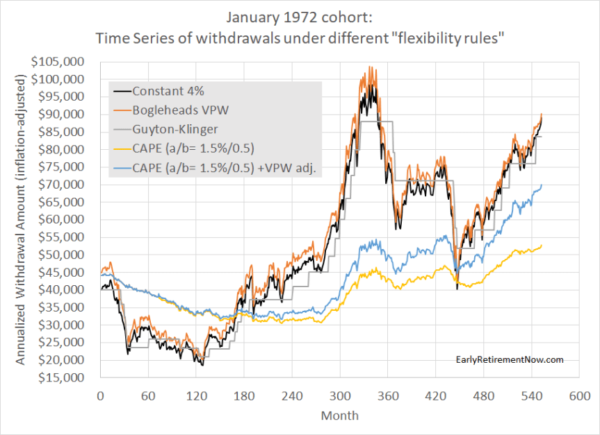
Case in point: The 1972 cohort! It suffered some of the same bad market environment as the 1966 cohort but by starting six years later you avoided some of the initial weak equity and bond returns. But due to the recessions in the 1970s/80s it still had a bad first decade before the great bull market of the 1980s and 1990s kicked in. Only, nobody knew that the big recovery was around the corner until later, so the 1972 cohort would have…
- …unnecessarily gone back to part-time work for about a decade.
- …unnecessarily slashed withdrawals under the Constant % Rule, VPW and Guyton-Klinger Rules, by up to 50%. Recovery only after 15 years!
- …unnecessarily walked down the withdrawals under the CAPE-based rules. Not quite as badly as with VPW, but the walk-down would have also lasted longer. 25+ years! Ouch!

How about the year 2000 cohort? The 2000 cohort is an interesting crowd because it’s not even obvious yet whether they will be a 4% Rule casualty or not. For a 30-year time horizon, we’ll have to wait until 2030 to find out! It is sometimes referred to as a 4% Rule success story, though I seriously doubt that, see Part 6 of this series! Well, just for the moment, let’s take the 4% fans by their word and assume that the 2000 cohort was a success. Well, let’s hope they didn’t follow the flexibility mantra because that would have meant going back to work for a total of around 9 years (50% rule) or 11 years (30% rule).

The other dynamic/flexible rules look equally unattractive. After 18 years, neither the Constant %, Bogleheads VPW nor the Guyton-Klinger Rules would have recovered to their initial withdrawal amounts. That’s despite the fact that the portfolio without the withdrawals would have easily recovered. But as I pointed out last time (Myth #2), the portfolio takes longer to recover if you take money out along the way. I’m almost too embarrassed to make this obvious and trivial point but you’ll be surprised how often people neglect this little detail…

The CAPE-based rules would have done pretty well, though. No noticeable decline in consumption. But then again, due to the nosebleed high CAPE Ratio in 2000, you would have withdrawn only slightly above 2.5% of the portfolio! So, here’s an example where flexibility would have worked. But only if you had accumulated a net worth of 40x consumption instead of 25x!
Myth #6: Social Security to the rescue!
Social Security, to be sure, can be a great addition to the early retirement planning. As I showed in my Case Study Series, many volunteers ended up with safe withdrawal rates North of 4%. Thanks to Social Security and pensions! For “older early retirees” Social Security can make a big difference. If you expect benefits worth $20k per year and have a $1,000,000 initial portfolio then the fail-safe withdrawal rates for 1929 and 1966 would have increased by this much, depending on when benefits start:
- Benefits start after 20 years: +0.45%
- 25 Years: +0.29%
- 30 Years: +0.20%
- 35 Years: +0.14%
- 40 Years: +0.08% (all figures calculated with the Google Sheet developed in Part 7)
It helps tremendously if you’re 50 years old and expect the maximum benefits at age 70, only 20 years into retirement. But for retirees in their early 30s, future Social Security benefits will likely not move the needle much. If the failsafe is somewhere around 3.25% (1929) or 3.50% (1966) without Social Security then Social Security doesn’t even get close to making that a 4%!
Myth #7: Thou shalt not over-accumulate wealth
I’m throwing this one in just to poke a little bit of fun at the flexibility fans. That’s because here I’m actually the one invoking flexibility while they seem to be surprisingly stubborn and inflexible. The criticism that I hear most often is that I’m overly conservative and will just end up with way too much money. My response: I could get rid of that problem pretty quickly, for flexibility is a lot easier when you have too much money:
- Give money to our church and a number of charities.
- Donate money to a university. We don’t have the cash to fund a building or a stadium named after us. But did you know that with a low seven-figure sum you can create an endowed professorship or chair at most universities? How cool would it be if we funded the “ERN Family Chair of Economics” at my alma mater? And if the university manages the money wisely that endowed chair might last longer than some football stadium, too! 🙂
- Help out our daughter with student loans, house down-payment, etc.
- Travel in more comfort: First class instead of coach class! A suite on the Queen Mary 2 instead of an interior stateroom on a Royal Caribbean cruise!
So, the possibilities are endless. And for all those who are still inflexible and uncreative about how to get rid of their extra cash, please reach out to us and I’ll let you know our checking account number! We can get rid of your excess cash problem!
Thanks for stopping by today! Please leave your comments and suggestions below! Also, make sure you check out the other parts of the series, see here for a guide to the different parts so far!
Picture Credit: pixabay.com
Yes, that is a bad summary bullet point by Jim Collins.
Earlier in Jim’s article he says “In fact, if you gave up the inflationary increases and took 7% each year you would have done just fine 85% of the time.” The Trinity study does say exactly this for a 30 year retirement in Table 1 for 100% stocks and no inflation adjustments. The Trinity study talks about a 7% withdrawal rate surprisingly often. But always in the context of no inflation adjusts or a relatively short retirement.
In summary, I don’t disagree with anything you’ve said here. But I’d hate for people to disregard Jim’s (largely) excellent advice because of one bad bullet point. Thanks for the article.
Not doing CPI adjustments when inflation is running at 10%+ is very different from today when it’s running at 2%. Because the withdrawals are not camparable across time when doing no CPI adjustments I simply wish the Trinity Study had never even mentioned this completely useless result.
If these flexibility rules do not perform that well, then just fit the flexibility rules to the existing data and simplify them a bit.
I would prefer rules that look at interest rates and current market performance. Because when the Fed raises interest rates bonds start to look better and better! Caveat: I am now SHORT 2-year bonds and making a killing. I will short the 2 year until the bond curve inverts. Then I will buy long term bonds and maybe some puts.
When the interest rates get slashed by the Fed again I will actually lever myself above 100% stock allocation! Wait for the recession to be declared over and pile into stocks. IB has really cheap leverage, so being 150% stocks or whatever will actually be really inexpensive when interest rates are low.
Have you tried flexibility rules with interest rates in mind?
I like global macro asset allocation, so what you are proposing is really heart-warming because that’s part of what I did for 10+ years in my previous career.
That said, it’s not what most people would consider flexibility. And FIRE people who subscribe to the passive investing only mantra will not be up for anything like this.
Flexibility rules to consider:
1. Market performance flexibility:
Assume a $1M portfolio, 100% equities. 4% initial withdrawal rate.
Year one: 10% (real) decline, withdrawals reduced 10% (3.6%)
Year two: 20% (real) increase, withdrawals increase 20% (4.32%)
2. One can also consider CAPE based withdrawal timing to try to squeeze out a few points. If CAPE is high, annual withdrawal at beginning of year (get the equity money out of the market); if CAPE low take the smallest amount more frequently to leave it in the market longer.
3. Also have you considered different equity allocations (total US market is not the same as small-cap/foreign/emerging markets)? Although SoR risk should be greater with more volatile instruments, an equity glidepath might have markedly improved long-term performance. Portfoliocharts.com does some wonderful simulations with different allocations and SWR/PWRs.
Thanks for the amazing work!
Nick
Thanks!
I did 1+2 already:
1 is the Constant 4% Rule (and the VPW, which is the same but with an adjustemnt for the time horizon)
2 is the CAPE-based rule, whcih I did both for 1.5%+0.5/CAPE as well as the same adjustment for the time horizon as in the VPW
3: I didn’t do that yet. I have only the international index data since 1970, not enough data to run the full study. But notice that international stocks tank just around the same time as the US market. See this post:
https://earlyretirementnow.com/2017/08/23/how-useful-is-international-diversification/
So, I doubt that international diversification will make much of a difference.
Big ERN, love the blog! I really appreciate all the great analysis and writing you do. It has been inspiring and thought-provoking!
I love this entire series. The flexibility entries as well as the glidepath entries stick out as easy to learn from and apply.
This post’s idea of a cash cushion to use if your investments go 20%+ underwater is great. Two questions on that:
1) Would combining a 60 to 100% stock glidepath with the cash cushion be an even better strategy than doing just a glidepath or just a cash cushion? Since both work separately so well, combining might be even more optimal, right?
2) I couldn’t find discussion around why 20% underwater is the the time to use the cash cushion. Did you run a few models of 0%, 10%, 30%, etc and find 20% performed the best?
Thanks so much for writing this blog! I appreciate you and your knowledge!
Thanks for the questions!
1: I haven’t simulated that yet but it sounds like it depends on whether you do the cash cushion ON TOP of the glidepath or whether you replace x% of GP bond share with cash. In the former you likely soften the fall from the bear market even a little bit more. In the latter I would think it doesn’t make that much of a difference.
2: I played around with the cutoff and 20% seemed to be the best tradeoff between reacting early enough but also not too early.
Cheers!
Thanks so much! I played around with it a bit today using your fantastic ERN SWR Toolbox v2.0 Glidepath Case Study sheet.
Looking at the 9/1929 cohort, if we had $1M with $50k in annual spend as the goal, we would see the following metrics for a) $200k cash buffer with $800k portfolio (starting at 60/40 allocation and gliding up) vs b) $1M portfolio (starting at 60/40 allocation and gliding up):
Avg Glidepath $458,877 $256,095
Min Glidepath $169,415 -$575,229
The cash buffer makes a HUGE difference. In fact, it survives the great depression! Although once things hit $169k (the minimum during the run), things would probably have been quite scary!
Not as big of a difference with the cash cushion on the 1/1966 cohort though:
Avg Glidepath $151,923 $133,084
Min Glidepath -$1,023,771 -$1,072,809
Slightly better performance with the cash cushion, but still decimated pretty quickly.
Nice! Thanks for doing this! I’m busy here with unpacking and home improvement projects! 🙂
What do you think about using I Bonds for the cash bucket strategy (to avoid annual interest income on a large chunk of cash)?
The two approaches I’m contemplating are 1) keeping the T-bills in a tax-deferred account and then (if needed) extracting the money by swapping the T-bills for stocks in the tax-deferred account (in the 0% long-term capital gain bracket) while simultaneously selling an equivalent amount of stocks in a taxable account, or 2) keeping the cash in (tax-deferred, by their nature) I Bonds in a taxable account.
I haven’t found a great way to compare the historical return of 3 month T-bills vs. I Bonds. I suspect this is possible on stlouisfed.org, but my FRED skills are lacking.
Great series!
I’m not very familiar with I bonds but I know that there’s a benefit to keeping them until maturity. But that renders them ineffective as a cash bucket asset, right? And keeping them untouched for such a long time you’ll likely be better off with equities.
Or maybe I’m misunderstanding the advantages of I Bonds???
No worries! I Bonds pay interest that’s roughly CPI-U plus a fixed rate on top that’s determined at purchase (and that fixed bonus rate is sometimes 0%). I think there are interest penalties if you redeem them in within a few years. The advantages are: 1) they’re inflation protected (with a 0% floor, unlike TIPS) and 2) you can defer taxes on interest until you cash in the bonds.
My thinking was that any potential interest penalties and income tax on interest when you cash them in would be palatable if you’re cashing them in during a huge market drop to avoid selling depressed equities.
Having a fixed rate component to I Bonds is a little worrisome, I suppose (what if rates spike after retirement but inflation/CPI-U is tame?). Probably better to stick to the closest thing to cash you can, as you did with 3-month T-bills in your example.
Side note: I think the benefit you’re remembering is for Series EE Savings Bonds (which are guaranteed to double in value, regardless of their initial fixed rate, once they mature, effectively giving you a floor on their interest rate around 3%–IF you can hold them to maturity).
Ah, OK, I confused that one with the EE bonds. Never mind.
Well, the current yield doesn’t look so bad, so yes, your plan looks pretty solid to me.
Mr. ERN, I really have enjoyed your blog. Regarding sequence risk and the fact that you use an historical simulation approach in your simulations, have you ever modeled what is described in this article? https://seekingalpha.com/article/4126426-practice-summary-managing-sequence-risk-optimize-retirement-income?page=2 Here is the study that the article refers to: https://www.cfapubs.org/doi/suppl/10.2469/faj.v73.n4.5/suppl_file/clare_faj_supplementaltables_2017.pdf Due to copyright, I won’t submit the copy of the study that I purchased. I’m particularly interested in whether you’ve modeled a simple trend following approach like the 10-month moving average (to determine when to get out of stocks completely and then back in), which is what is simulated in the study. According to the authors of the study, the trend-following approach significantly improves outcomes (in terms of mitigating sequence risk, resulting in being able to use a higher withdrawal rate) than a buy-and-hold strategy. Since, in this post, you are zeroing in on 1929 and 1966 as your simulation starting points — and since you have already done the fine work of creating a simulation engine — I figure that you might be curious to see how sequence risk for these two cohorts would be affected. I recognize that using a simple trend-following algorithm is a less passive investing approach than, say, annual rebalancing to maintain a consistent mix of stocks and bonds…or using a glide path approach (and some Bogleheads who read this blog might scream bloody murder at my suggestion of a trend following algorithm), but I figure that the selection of a stock-bond mix or defining a glide path (which you’ve discussed in your various posts) still involves looking to the past to see what had produced a more optimal outcome, so I see no reason why looking at an alternative like trend following when simulating past returns would be any different.
Just like you, I’m very fascinated by momentum/trend signals. I’ve written about this approach here:
https://earlyretirementnow.com/2018/04/25/market-timing-and-risk-management-part-2-momentum/
I haven’t gotten around to writing up a post on how this would affect the SWR. My results from the historical simulations seem promising, so this confirms the results from the article. So, if you can muster the discipline of keeping up with this momentum signal you’d be able to hedge a little bit against Sequence Risk. Not sure if this will stay like tha in the future but it certainly worked well in the past!
I think your discovery with the cash buffer is seriously understated! I’ve read your whole series and it really jumps out at me. So the “4%” rule stands if you have an additional 10% cash buffer to insure against SRR (more like a 3.6% rule)? Do you have a spreadsheet that lets you play with this cash buffer and trigger percentage? If it’s in the google sheet you posted, I couldn’t find it. Thank you for all this great material!
Please see Excel file here:
https://drive.google.com/file/d/15QO1P0s9eI_8HaHtXpzvH77k8YtBHtse/view?usp=sharing
The cash buffer calculations in each of the year tabs (e.g., 1929, 1958, etc.) in columns Q through X. Hope this helps. 🙂
Could you please make that spreadsheet public? I can’t access it. Thank you!
Try if this one works:
https://earlyretirementnow.com/wp-content/uploads/2020/11/SWR-Part-25-Calc.xlsx
Alternatively, try this one:
https://earlyretirementnow.com/wp-content/uploads/2020/11/SWR-Part-25-Calc.xlsx
For some reason Google Drive doesn’t like storing MS Excel Files…
Hi ERN,
I share the view above that “the cash buffer [approach] is seriously understated!” — it’s almost like you are including it grudgingly. :-p
The issue is that it is difficult to model with the tools on the internet (simFire, etc. don’t allow a decision-rule based approach for when to use or re-fill the cash). It would be great if you made a post with your heat map Excel tables on the topic: failure rates vs. withdrawal rate vs. amount stashed away. I’m willing to bet that it would not cost so much extra cash to get to, e.g., 5% and 1% failure at thirty years!
vielen Dank!
Sean
Not sure how you would get to 5% WR. With the ADDITIONAL cash you can not get to 5% is the WR is expressed as withdrawal over the TOTAL portfolio. Maybe if you use the withdrawal over the non-cash portfolio only, But for withdrawals as percentage of stock+bond+cash portfolio, you will have a hard time getting above 4%.
Thank you for your replies! Yes, I’ve started to hack around in your spreadsheets, and that extra percent would be a long, long road. I would like to see more analysis on this “cash reserve to be used when the market drops 20%” sort of scenario. I do get the sense that this is a good tool to mitigate SWR.
Yes, if you start retirement at the most inopportune times (1929, 1960s, etc.) then if you had some cash on the sideline and live through the bear market and avoid liquidating equities at the bottom it helps. Somewhat. As I showed in Part 25. But it’s no panacea either! 🙂
What about using a savings/bucket strategy and refilling the savings using extra wealth accumulated in over-performing years?
Also have you looked into optimizing your portfolio itself toward a higher withdrawal rate? Instead of a simple 80/20 portfolio, (for example) how about mixing in some gold to skirt some volatility from stocks/bonds, maybe some small caps to speed up rebounds, REITs for further diversification from traditional stocks and for (relatively) steady income, etc, etc…
Gearing your portfolio to a high (historical) safe withdrawal rate paired with other strategies, like the savings/bucket may provide return rates above 4%.
I am very suspicious about back-ward optimizing the portfolio. You would load up on small-cap and value stocks because that worked well historically. But that really sucked recently.
I did cover gold as a hedge in Part 34.
REITs: not enough history.
I modeled the cash bucket strategy as mentioned in the post.
I modeled this as not being refilled because in the really bad scenarios you will not even have that “extra wealth” to replenish the bucket.
Given financial repression, might you could re-run your analysis assuming the cash bucket DOES reduce the bond investment in the portfolio?
Could one protect an otherwise 100% stock portfolio with a three year cash bucket?
Thanks.
You mean do a glidepath from, say, 60% stocks, 20% bonds, 20% cash to 60% stocks, 40% bonds?
Proabbly doesn’t help becasue cash doesn’t offer the diversification from the duration effect. But might have helped in the 1970s.
3 years cash is way too little with an othersie 100% stock portfolio.
I appreciate the reply, ERN.
I mean I’d like to see a like-to-like comparison: a $1M 80/20 stock/bond portfolio compared to something like a $1M 80/(20 – 3 years cash)/3 years stock/bond/cash bucket portfolio, where the cash is only withdrawn if the investment portfolio goes more than 20% underwater, and once exhausted never replenished.
I say something like because I’d be real curious if the optimal portfolio might exclude bonds today? Really struggling to see their value.
How many years cash would a stock/cash bucket portfolio need have? Five, maybe?
Thanks again.
We can come up with all sorts of intricate strategies that would have “worked” in past episodes. But it sounds lie overfitting that might backfire in the next, slightly different episode.
5 years worth of safe assets would not have been enough in some of the past bear markets where it took 10+ years for the stock market to recover.
And again: bonds have a purpose due to the negative correlation with stocks during many past bear markets. Negative correlation (bonds) > zero correlation (cash/money market).
Sure (overfitting).
I guess unstated was my assumption that a bear market lasting over 3 years would scare anyone from much discretionary spending, so the original 5 years cash would last longer. Not 10+ years though, no.
But bonds have interest rate risk which cash does not. And negative correlations might not hold if we enter stagflation as a result of the very financial repression that holds interest rates below the rate of inflation today.
That aside, do you favor long-term treasuries for portfolios with high equity allocations as they the most negatively correlated?
Thanks.
If the interest rate risk is negatively correlated with your stock portfolio (bonds gain when stocks go down) then it’s a risk I am willing to take. That was the case in the last 4 recessions.
I model my simulations with intermediate bonds (10y). Longer duration offers even more diversification.
Thanks again.
Thinking I’ll likely shift to 80/10/10 stocks/long-term treasuries/cash, and withdraw from the cash only as you suggest (portfolio -20%, never replenish).
Bonds may no longer derisk a portfolio, but hopefully they’ll continue to diversify.
Sounds like a plan. But don’t discount bonds too much. If we have anouther bad recession, I’d rpredict the 10y yield goes to 0 and you do get a boost from the duration effect.
Revisiting this, any chance you would you could re-run your analysis assuming the cash bucket is not in addition to the starting value, but rather included?
For example, assuming a starting value of $1M and $40K/year expenses, setting aside three year’s expenses would look like: $880K portfolio, $120K cash bucket.
1 How many year’s expenses would one need set aside in the cash bucket?
2. Given the cash bucket, how much does the makeup of the portfolio itself matter?
Thanks.
That’s all a matter of scaling. $880k in the portfolio and $120k in the cash bucket means that you have only 3Y in cash and the rest of the portfolio has to sustain a withdrawal rate of 40/880=4.54%. Seems pretty risky.
Thanks so much for all your blog posts – I’ve read many of them! As variation of “3.25% initial withdrawal rate (=floor) plus upward adjustments”, can one simply “re-retire” at 3.25% SWR whenever that would raise the withdrawal amount?
For example, say you start with $1,000,000, taking out $32,500. The market does well at first and the portfolio goes up to $1,100,000, so you “re-retire” on $35,750 per year. Then the market tanks and the portfolio is at $900,000, but you keep your current withdrawal rate ($35,750 + inflation adjustments). After some time the portfolio has recovered again so that 3.25% of it is more than your current withdrawal amount, so you retire a third time at 3.25% of the portfolio value at the time. And so on…
Obviously each time you “re-retire” like this your probability of failure (running out of money) increases compared to sticking with “the original retirement”, but is this a safe enough approach if you do it with a truly “safe” SWR (“TSWR”? :)), like 3.25% or even lower? It would be interesting to see what withdrawals rates you would have ended up with histortically, too.
You would eventually reach the market all-time-high that will have a low SWR, comparable to 1929 or 1965. But if you set the WR low enough, sure, you will do well with this approach.
I suppose the question then is: how low is low enough? How much of a margin of safety do you need compared to the historically safe SWR (3.25%?) In practice, I’d probably not increase my WR as much as I possibly could, e.g. if the portfolio doubled in value I’d probably not start withdrawing 6.5% of the original amount pa, but maybe 5%.
The historical worst case WR is what you’d target and you’d not run out of money unless the future is worse than what we observed in the past.
Hi Big ERN, loving this series.
I would liks your opinion on 3 SWR strategies you suggest:
1. 3.25%
2. 1.5% + 0.5 CAEY.
As Shiller CAPE is currently 39.70 (let’s call it 40), that would be 2.75% (with potential to increase if CAEY increases, as opposed to 3.25% flat).
3. 25 years of 80/20+ 3 years of cash as you suggested above (I rounded up 120k) means total net worth that equals to 28 years of exepnses from which we can withdraw 1/28= 3.57% (in the order you described of course).
I understand that method 2 starts lower but can increase but if there’s a way to make 3.57% work in the worst-case scenarios, why stick to 3.25%?
Correct.
Alsp notice that the CAPE is calibrated for asset preservation. You can still amortize the or slowly deplete your assets and likely up the SWR to about 3.75%.
Thanks! The preservation/depletion was my missing piece to understand this.
Thank you so much for all of your work ERN, as I approach my big RE date I am rereading a lot of your SWR series. I wonder if you have looked at the Vanguard Dynamic Spending model. I think the key is having a minimum spend amount, so that even though you get the wild swings in your withdrawal rate over time you have a pre-set minimum. The Vanguard paper does not mention a minimum withdrawal amount but it is an option on FICalc app and when I used the parameters of starting rate of 3.6%, increase ceiling of 25%, decrease floor of 2.5% and a minimum spend of the amount that would be equivalent to 3.15% of my initial portfolio (which is inflation adjusted) it survived a 50 year retirement.
Adding a minimum spend to the fixed percent of portfolio also worked. With this I used a fixed 4% of the portfolio each year but once again added the 3.15% minimum spend.
I like that both of these make it easy to determine your spend amount each year and with their dynamic nature you get to benefit from when the market is up but when it is down you don’t go below a predetermined amount, since those super low lows where the problem with most of the dynamic spending models.
I would love to know what you think about this option.
You can add all sorts of bells and whistles. But note that with a min spend amount you might run out of money eventually, while the CAPE-based model will never do so. It’s all about tradoffs. You cannot magically create superior results without any drawbacks.