


Update 8/29/2018: Check out Part 28 as well with some enhancements to the Google Sheet!
Update: We posted the results from parts 1 through 8 as a Social Science Research Network (SSRN) working paper in pdf format:
Safe Withdrawal Rates: A Guide for Early Retirees (SSRN WP#2920322)
One commenter the other day had a good suggestion: Publish the Excel spreadsheet that we use in our safe withdrawal rate research. Great idea! There is only one problem: we didn’t use Excel to calculate any of the SWRs. We did use Excel to create some tables, but the computation and most charts were all done using GNU Octave, a free number-crunching programming language, similar to Matlab.
But we still liked the idea of creating a tool to run some quick SWR calculations. In Octave, we can calculate a large number of simulations and calculate safe withdrawal rates over a wide range of parameter value assumptions. Millions and millions of SWRs over many different combinations of parameter values (retirement horizons, final asset value target, equity shares, other withdrawal assumptions). That would have been cumbersome, probably even impossible to implement in Excel. But a quick snapshot on how one single set of SWR parameters would have performed over time? That’s actually quite easy to do, even though there are 1,700+ different retirement cohorts between 1871 and 2015.
Here’s the Google Sheet Link:
Link to the EarlyRetirementNow SWR Toolbox v1.0
For obvious reasons, the baseline Google Sheet can only be edited by us. If you like to run your own calculations you have to download your own copy. There are at least two ways to do so:
- (recommended) Click on Menu, then “Make a Copy” or “Add to MyDrive” to get a local copy of the spreadsheet in your own GoogleDrive. You can then edit the sheet and use your own assumptions.
- Click on Menu, then “Download as” then “Microsoft Excel (.xlsx)” to get a copy as an Excel file to store on your own hard drive. It’s not really recommended because most of the formatting will get lost. But if you care only about the computations you should be fine.
Update February/March 2017: Gold and cash returns
- Gold returns are only completely trustworthy after 1968 when I got the London Fixing time series via Quandl. Before that, I had to rely on annual data from OnlyGold.com. If someone has a better (monthly) time series for 1871-1967 please let me know!
- For cash returns I use:
- 3-month T-bill interest rates from the Federal Reserve starting in 1934. Monthly data.
- I have annual data going back to 1928 from NYU-Stern. Data gathered via Quandl.
- For 1871-1927 I use annual data on 1-year T-bill yields from Prof. Rober Shiller. It’s not exactly ideal to splice it this way but it’s the best I can right now. If someone has better data, please let me know!
How our tool is different from cFIREsim
- We use monthly data, while cFIREsim uses only annual data.
- We project forward return forecasts beyond 2016 year-end so we can calculate SWR for more starting dates. For example, the January 2000 cohort is already far underwater, as we showed a case study last week. Even aggressive return assumptions will still wipe out the portfolio before too long and we like to count those cohorts as 4% SWR failures even before the utter failure is actually confirmed.
- cFIREsim asks you for a specific withdrawal rate and then simulates how that rate would have performed over time for each of the different starting dates. We go the opposite route: We specify a final value target and our spreadsheet calculates the exact initial withdrawal rate that would have precisely matched the final value target. For every retirement cohort between February 1871 and December 2015 (=1,739 months). The advantage of this procedure is that we can then easily calculate the failure rates of different initial SWR without calculating any new simulations. The failure rate of the 4% rate? Simply calculate the share of ERN-SWRs that are greater than 4%. And redo the same for all rates between 3.00% and 5.00% without ever calculating any new set of simulations as would have been required in cFIREsim.
Enter Parameters
Fields with the orange shading are asking for user inputs:
- The Equity share. We are aggressive and set this to 90%. The residual is invested in 10-year U.S. Treasury Benchmark Bonds.
- The expense ratio: We currently set it to 0.05% p.a. One-twelfth of this is subtracted from each month’s return.
- Equity projected returns post 12/31/2016. These are real annualized return assumptions. In our SWR simulations we set this to 6.6% but here we are a bit more cautious and set this to a more conservative 5.0%.
- Bond returns: for the near-term (notice how low current 10Y yields are) and then longer-term. Short-term we use only 0.5% over the next ten years, then going a bit higher to 2.0% real return after that.
- Same for Cash: We expect pretty low cash returns over the next 10 years (0% real) and then a bit of a bump after that (+1% real).
- Expected future real return for Gold: We set this to +1%. Historically, gold has returned only about 1.5% p.a. after inflation.
- The length of the retirement horizon in months (e.g. 60 years = 720 months)
- The target final asset value as % of the initial portfolio. We set this to 50%.


Below the main parameters, you can also set an entire time series of additional cash flow needs (all monthly numbers as % of the initial portfolio value). For example, we predict to get a pension and Social Security worth about 1% of the initial net worth (in 2018 dollars) 25 years into retirement. So, starting in month 301 we set this value to 1%/12=0.0833%.


That’s all you need. The computer does the rest for you. It calculates the safe withdrawal rates for each month starting in February 1871 to December 2015 that would have exactly matched the final value targeting the last month of the retirement horizon.
Results
Some summary tables are in the first tab “Parameters & Main Results.” Be patient, depending on the internet connection and computer speed it may take a few seconds to recompute all results!
In the table on the left, we calculate the failsafe safe withdrawal rate both over the entire sample and for retirement cohorts post-1950 as well as the 1st, 5th, and 10th percentile. For example, since 1950, a 3.61% withdrawal rate would have failed 5% of the time and succeeded 95% of the time.
On the right, we calculate the failure probabilities of specific rates between 3% and 5% in 0.25% steps, again over the entire sample and since 1950, but also in the three CAPE regimes (<20, 20 to 30 and 30+). In the CAPE 20-30 regime, notice the big jump in the failure rates once you go beyond 3.5%!


We also throw in a chart with the data in the right table:


Distribution of the final portfolio value
In the tab “Distribution of Final Value” we can also specify a withdrawal rate and see the distribution of final asset values (real, CPI-adjusted, as multiples of initial). In the example below, we use the 4% rule. We are mostly worried about the left side of the distribution, so final values between the minimum and median. Note how for the median retirement cohort the investor would have grown the portfolio to 8 times (!) its initial real value. The maximum final value would have been a staggering 62-times the initial value. But at the same time, almost 10% of the retirement cohorts ran out of money!


More results
Also make sure you check out the tab “SWR time series,” which includes the SWR for all 1,700+ months in the simulation. For a quick look, there’s a time series chart as well. Notice how there are quite a few times when the SWR is quite substantially below 4%!


How the hell do we calculate so many SWRs?
Or, in other words, where’s the mega-spreadsheet that has 1,700 rows and 720 columns to iterate over the 60 years worth of portfolio values for the 1,700+ cohorts? We don’t need any of that! The withdrawal rate arithmetic is much easier than that. Stay tuned for next week’s post: our technical appendix with some of the background on the withdrawal rate arithmetic we developed. But if you’re interested, check out how the SWR tab “SWR time series” in Column E are calculated through some pretty trivial calculations from just four auxiliary variables in the tab “Stock/Bond Returns,” columns L through O. Likewise, we calculate the final asset values for the fixed withdrawal rate (column F in that same tab) without ever iterating over 720 months of returns each time we change the withdrawal rate. Much more elegant than the brute-force method in cFIREsim!
Case Study:
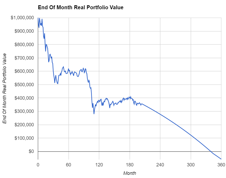
As we just mentioned, in calculating the SWR we never even go through the cFIREsim-style exercise of iterating over months and years and plotting the portfolio value time series. That would be too cumbersome for all 1,739 retirement cohorts and several decades of retirement horizon. But if you were wondering how any particular withdrawal rate would have performed over time for one specific retirement cohort, here’s the way to do it. Check out the tab “Case Study” where we can add the parameter values, again the orange shaded fields: The retirement start date (year/month), initial portfolio value and the withdrawal rate. And the computer does the rest!


The time series of portfolio values is in column D and also in the time series chart. This will use the same portfolio allocation and also the same supplemental income/expenses as in the main parameter tab. As we already noted last week, January 2000 would have been a pretty bad starting date for retirees. Not just early retirees!

Disclaimers
Please read the disclaimers here on the website and in the Google Sheet. We gladly grant the right for others to utilize our work but please make sure to credit us and quote us properly. We do own the copyright to everything we post here!
Also, note what this toolkit is and what it isn’t: It is a toolkit to determine how different withdrawal strategies would have performed in the past. It’s not a forecast. Past results are no guarantee of future results! But we can still learn from the past.