


One of the most requested topics for our Safe Withdrawal Rate Series (see here to start at Part 1 of our series) has been how to optimally model a dynamic stock/bond allocation in retirement. Of course, as a mostly passive investor, I prefer to not get too much into actively and tactically timing the equity share. But strategically and deterministically shifting between stocks and bonds along a “glidepath” in retirement might be something to consider!
This topic also ties very nicely into the discussion I had with Jonathan and Brad in the ChooseFI podcast episode on Sequence of Return Risk. In the podcast, I hinted at some of my ongoing research on designing glidepaths that could potentially alleviate, albeit not eliminate, Sequence Risk. I also hinted at the benefits of glidepaths in Part 13 (a simple glidepath captures all the benefits of the much more cumbersome “Prime Harvesting” method) and Part 16 (a glidepath seems like a good and robust way of dealing with a Jack Bogle 4% equity return scenario for the next 10 years).
The idea behind a glidepath is that if we start with a relatively low equity weight and then move up the equity allocation over time we effectively take our withdrawals mostly out of the bond portion of the portfolio during the first few years. If the equity market were to go down during this time, we’d avoid selling our equities at rock bottom prices. That should help with Sequence of Return Risk!


So, will a glidepath eliminate or at least alleviate Sequence Risk? How much exactly can we benefit from this glidepath approach? For that, we’d have to run some simulations…
Background on glidepaths
Target date funds use a time-varying asset allocation depending on the participant’s age. The idea is that young investors can and should take on more risk and hold a higher portfolio share in equities. Then, as retirement approaches, investors shift more into bonds to reduce risk. In fact, you don’t even have to do this shift yourself; Vanguard or whoever your provider may be will do it for you! Here’s Vanguard’s take on the glidepath, see chart below. The equity share (domestic plus international) in their target date funds starts at around 90%, drops to around 50% at the traditional retirement age of 65 and then further drops to 30% by age 72.


But recent research has shown that Vanguard (and many other providers of target date funds) actually got it wrong, at least for the post-retirement glidepath. The glidepath of equity weights should ideally start to increase (!) again once you retire. Michael Kitces wrote about this topic (on his blog here and here and in an SSRN working paper joint with Wade Pfau) and proposed to keep the minimum equity share at or around the retirement date before starting to raise the equity weight again during retirement.


The rationale is that the rising equity glidepath in retirement would be insurance against sequence of return risk. After all, the number one reason retirees run out of money is bad returns during the first few years of retirement. A low equity allocation shields you from short-term equity volatility, but longer-term you will need the high equity share to make it through 40, 50 or even 60 years of retirement. So, a dynamic stock/bond share would thread the needle to achieve both long-term sustainability and short-term protection.
Of course, as with all of the traditional retirement research, it has limited use for the early retirement community. My experience has been that a lot of the research targeted at the traditional retirement crowd, calibrated to capital depletion over a 30-year horizon, is less applicable to the FIRE crowd. For example, Safe Withdrawal Rates have to be lower over a 60-year horizon than over a 30-year horizon. And, equally important, equity weights have to be higher over a 60-year horizon to ensure long-term sustainability. Case in point, the 30% equity weight at the retirement start and 60% in the long-term as indicated in the Kitces chart above would be way too low for early retirees!
So, when unhappy with the whole Kit(ces) and Caboodle of hand-me-down research, what am I supposed to do? If you want something done and done right, you just have to do it yourself! That’s where the Big ERN simulation engine comes in handy!
Simulation assumptions:
- Monthly data from January 1871 to July 2017.
- A 60-year retirement horizon.
- Retirement dates from January 1871 to December 2015 (with extrapolations using conservative return forecasts for bonds and stocks beyond July 2017).
- Final value targets of 0% (Capital Depletion), 50% of the initial real value and 100% of the initial portfolio (in real terms).
For each of the 1,700+ cohorts, we calculate the safe withdrawal rate, i.e., the initial withdrawal percentage that exactly achieves the final target value after 60 years, assuming withdrawal amounts are adjusted for CPI-inflation regardless of the portfolio performance. As usual, we calculate the SWRs for the 21 different static Stock/Bond allocations (0% to 100% stocks in 5% increments). But we also simulate a total of 24 different glidepaths, comprised of the different combinations of glidepath parameters:
- Two different end points: 80% and 100%. Why not lower end points? As we will see later, the long 60-year retirement horizon necessitates a much higher (long-term) equity weight than the often-quoted 60% or even 50%.
- Three different starting points: 20, 40 and 60 percentage points below the end point.
- Two different slopes. Notice that I had to increase the slopes for the glidepaths that cover more ground, otherwise, the transition would take way too long:
- 0.2% and 0.3% per month for the glide paths starting 20 percentage points below the max,
- 0.3% and 0.4% for the paths starting 40 percentage points below the final target,
- 0.4% and 0.5% per month for the paths that start 60 percentage points below the final target.
- Two different assumptions for the glidepaths: Passive vs. Active
- Passive means that we stubbornly increase the equity weight every month by the slope parameter.
- Active means that we increase the equity share only when equities are “underwater,” i.e. when the S&P500 index is below its all-time high. We want to avoid shifting out of bonds too early, i.e., before the market peak and then having insufficient bond holdings when equities take a dive.


The “active” glidepaths, of course, are dependent on the retirement cohort. The transition from, say 60% to 100% equities would take a little bit longer depending on how equities perform during that time, see a sample of active glidepaths for the January 1965 to January 1980 cohorts below:


Results:
Let’s start with the failure rates of our preferred safe withdrawal rate, 3.50%. In the chart below, I plot the failure rates of three static equity weights, 60%, 80%, 100%, as well as the various glidepaths. Those with a final equity weight of 80% at the top and with a final equity weight of 100% at the bottom. First, let’s do this for all 1,700+ monthly retirement cohorts regardless of equity valuations (“All CAPE”):


Some patterns emerge from this chart:
- There will be at least a few glidepaths with lower failure rates than the static allocations. It seems that the 80% to 100% and 60% to 100% glidepaths deliver consistently lowest failure rates, regardless of the final value target!
- Who would have thought that the maximum long-term equity weight delivers the lowest risk? This goes back to the superior equity long-term expected returns; once you make it through the shaky first 5-10 years exposed to sequence risk you want to max out the equity weight!
- The very long transitions over 60 percentage points (20 to 80% and 40 to 100%) tend to be pretty consistently inferior to the other glidepaths. The 20 to 80% glidepaths are even inferior to the static 80% and 100% allocations! Apparently, the initial stock weight was too low and/or the transition took way too long (even with the accelerated slopes of 0.4% and 0.5%!)
Do glidepaths become more useful when the Shiller CAPE is high?
As we have pointed out numerous times before (for example, in Part 3 of the series), the Shiller CAPE is strongly correlated with safe withdrawal rates. Plain and simple: Sequence of Return Risk is elevated when the CAPE ratio is high! Is that also reflected in the glidepath performance? You bet, see chart below:


- First, notice that the failure probabilities of the static rules are now much higher due to the higher CAPE ratio. Even a capital depletion target fails with about 17%, 7% and 12% probabilities for the static equity weights of 60%, 80%, and 100%, respectively.
- Most glidepaths pretty consistently beat the static equity weights. The consistently best performers are the 60 to 100% glidepaths and the active glidepaths perform slightly better than the passive ones. The failure rates are less than half those in the static allocation simulations!
- The 20 to 80% and 40 to 100% glidepaths are still inferior to the other glidepaths. And the 20 to 80% glidepaths are inferior to the even the static asset allocations.
More on the distribution of SWRs: Failsafe and other SWR percentiles
A lot of very risk-averse retirees like to set their SWR to the failsafe SWR in historical simulations. That seems very conservative, but I can see where they are coming from. If your strategy would have handled the Great Depression, the nasty 1970s/early 1980s, and the volatile 2000s you can probably also use it in 2017 without too much worry!
In the table below, I calculate the failsafe SWR, i.e., the minimum historical safe withdrawal rate (60-year horizon, 0% final value), as well as some other percentages (1st percentile, 5th, 10th and 25th). So, for example for the 80% fixed equity allocation, the absolute lowest historical SWR would have been 3.14%. A 3.43% initial SWR would have failed 1% of the time, 3.59% would have failed 5% of the time, 3.86% would have failed 10% of the time and 4.48% would have failed 25% of the time. I don’t think planning for a 25% or even 10% failure probability is very prudent – personally, I try to target a failure probability in the single digits, e.g., 5% – but I display the numbers just in case someone wonders.
The left portion of the table is for all possible retirement start dates (about 1,700 of them, monthly data from 1871 to 2015). The right part of the table is for those months when the Shiller CAPE ratio is above 20. In the top portion of the table, I also marked with green boxes the maximum value among the static asset allocation rules in each column. Notice how the maximum in each column is at between 75 and 100%! To make it through a 60-year retirement, you can’t have a 60% or even 50% equity share. That only works for 30-year horizons! Also notice that with a CAPE>20 all numbers in the far right column are <4%, so the 4% had a failure rate of over 25% regardless of the equity glidepath!


In any case, 60 to 100% glidepaths generate the consistently best SWRs. For the über-conservative FIRE planners who are looking for the failsafe 60-year SWR conditional on our current 20+ CAPE environment, a fixed 75% stock allocation would allow a withdrawal rate of only 3.25% and that’s already the max over the static allocation paths! The 60 to 100% glidepaths would have allowed between 3.42 and 3.47%. That’s an improvement of between 0.17% and 0.22%. It doesn’t sound like much but it’s an improvement of between 5 and 7% of annual withdrawals. Not bad for doing a simple glidepath allocation.
Likewise, if I’m OK with a 5% failure probability conditional on a CAPE>20, then the static stock allocation of 80% would give me an SWR of 3.47%. The glidepaths would have allowed between 3.57% and 3.63%. Only an additional 0.16%, but that’s about 5% more consumption every year!
So, we won’t get all the way to 4%, but we bridge about one-third of the way, simply by playing with the asset allocation over time.
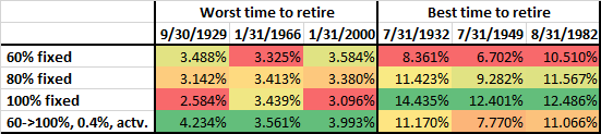
A small caveat, though; the calculations raise the question: do we get something for free? Is this some sort of a money-making arbitrage machine? Of course not! A glidepath will deliver a higher safe withdrawal rate if you have an equity drawdown early on in retirement. But the opposite is true as well. That 60 to 100% glidepath that performed so well during the major Sequence of Return Risk disasters will also underperform if stocks rally during the first few years of retirement. Let’s look at the table below that displays the SWRs of the 60%, 80% and 100% static equity weight and the 60 to 100% glidepath with a 0.4% monthly slope conditional on equity performance. As we already know, it beats the static equity allocation rules significantly when retiring at the market peaks (=worst time to retire). But the glidepath also falls significantly behind the 100% equity allocation if you were to retire at one of the three market bottoms (=best time to retire). It handily beats the constant 60% allocation and is slightly inferior to the 80% constant equity allocation. But I wouldn’t really care too much about falling behind in that case. You still get phenomenal SWR, just a little bit worse than the even more phenomenal SWRs of the 100% equity allocation.

Conclusion
Early retirees need the power of equity expected returns to make the nest egg last for many decades. Even more so than the traditional retiree at age 65! But that exposes us to Sequence of Return Risk. An equity glidepath can alleviate some of the negative effects of Sequence of Return Risk. But it shouldn’t come as a surprise that you will never completely eliminate the risk. For a given withdrawal rate, say 3.5%, we can only reduce the failure rate while leaving some residual risk. And likewise, the 4% rule would still not be safe for today’s early retirees even with an equity glidepath.
Moreover, an equity glidepath is like an insurance policy. A hedge against a tail event! On average it will cost you money, but if and when you need it the most it will likely pay off. Exactly when the static stock/bond allocation paths had their worst sustainable safe withdrawal rates you get slightly better results but you also give up some of the upside if the equity market “decides” to rally some more right after your retirement. But that’s a good problem to have!