
One of the most requested topics for our Safe Withdrawal Rate Series (see here to start at Part 1 of our series) has been how to optimally model a dynamic stock/bond allocation in retirement. Of course, as a mostly passive investor, I prefer to not get too much into actively and tactically timing the equity share. But strategically and deterministically shifting between stocks and bonds along a “glidepath” in retirement might be something to consider!
This topic also ties very nicely into the discussion I had with Jonathan and Brad in the ChooseFI podcast episode on Sequence of Return Risk. In the podcast, I hinted at some of my ongoing research on designing glidepaths that could potentially alleviate, albeit not eliminate, Sequence Risk. I also hinted at the benefits of glidepaths in Part 13 (a simple glidepath captures all the benefits of the much more cumbersome “Prime Harvesting” method) and Part 16 (a glidepath seems like a good and robust way of dealing with a Jack Bogle 4% equity return scenario for the next 10 years).
The idea behind a glidepath is that if we start with a relatively low equity weight and then move up the equity allocation over time we effectively take our withdrawals mostly out of the bond portion of the portfolio during the first few years. If the equity market were to go down during this time, we’d avoid selling our equities at rock bottom prices. That should help with Sequence of Return Risk!

So, will a glidepath eliminate or at least alleviate Sequence Risk? How much exactly can we benefit from this glidepath approach? For that, we’d have to run some simulations…
Background on glidepaths
Target date funds use a time-varying asset allocation depending on the participant’s age. The idea is that young investors can and should take on more risk and hold a higher portfolio share in equities. Then, as retirement approaches, investors shift more into bonds to reduce risk. In fact, you don’t even have to do this shift yourself; Vanguard or whoever your provider may be will do it for you! Here’s Vanguard’s take on the glidepath, see chart below. The equity share (domestic plus international) in their target date funds starts at around 90%, drops to around 50% at the traditional retirement age of 65 and then further drops to 30% by age 72.

But recent research has shown that Vanguard (and many other providers of target date funds) actually got it wrong, at least for the post-retirement glidepath. The glidepath of equity weights should ideally start to increase (!) again once you retire. Michael Kitces wrote about this topic (on his blog here and here and in an SSRN working paper joint with Wade Pfau) and proposed to keep the minimum equity share at or around the retirement date before starting to raise the equity weight again during retirement.

The rationale is that the rising equity glidepath in retirement would be insurance against sequence of return risk. After all, the number one reason retirees run out of money is bad returns during the first few years of retirement. A low equity allocation shields you from short-term equity volatility, but longer-term you will need the high equity share to make it through 40, 50 or even 60 years of retirement. So, a dynamic stock/bond share would thread the needle to achieve both long-term sustainability and short-term protection.
Of course, as with all of the traditional retirement research, it has limited use for the early retirement community. My experience has been that a lot of the research targeted at the traditional retirement crowd, calibrated to capital depletion over a 30-year horizon, is less applicable to the FIRE crowd. For example, Safe Withdrawal Rates have to be lower over a 60-year horizon than over a 30-year horizon. And, equally important, equity weights have to be higher over a 60-year horizon to ensure long-term sustainability. Case in point, the 30% equity weight at the retirement start and 60% in the long-term as indicated in the Kitces chart above would be way too low for early retirees!
So, when unhappy with the whole Kit(ces) and Caboodle of hand-me-down research, what am I supposed to do? If you want something done and done right, you just have to do it yourself! That’s where the Big ERN simulation engine comes in handy!
Simulation assumptions:
- Monthly data from January 1871 to July 2017.
- A 60-year retirement horizon.
- Retirement dates from January 1871 to December 2015 (with extrapolations using conservative return forecasts for bonds and stocks beyond July 2017).
- Final value targets of 0% (Capital Depletion), 50% of the initial real value and 100% of the initial portfolio (in real terms).
For each of the 1,700+ cohorts, we calculate the safe withdrawal rate, i.e., the initial withdrawal percentage that exactly achieves the final target value after 60 years, assuming withdrawal amounts are adjusted for CPI-inflation regardless of the portfolio performance. As usual, we calculate the SWRs for the 21 different static Stock/Bond allocations (0% to 100% stocks in 5% increments). But we also simulate a total of 24 different glidepaths, comprised of the different combinations of glidepath parameters:
- Two different end points: 80% and 100%. Why not lower end points? As we will see later, the long 60-year retirement horizon necessitates a much higher (long-term) equity weight than the often-quoted 60% or even 50%.
- Three different starting points: 20, 40 and 60 percentage points below the end point.
- Two different slopes. Notice that I had to increase the slopes for the glidepaths that cover more ground, otherwise, the transition would take way too long:
- 0.2% and 0.3% per month for the glide paths starting 20 percentage points below the max,
- 0.3% and 0.4% for the paths starting 40 percentage points below the final target,
- 0.4% and 0.5% per month for the paths that start 60 percentage points below the final target.
- Two different assumptions for the glidepaths: Passive vs. Active
- Passive means that we stubbornly increase the equity weight every month by the slope parameter.
- Active means that we increase the equity share only when equities are “underwater,” i.e. when the S&P500 index is below its all-time high. We want to avoid shifting out of bonds too early, i.e., before the market peak and then having insufficient bond holdings when equities take a dive.

The “active” glidepaths, of course, are dependent on the retirement cohort. The transition from, say 60% to 100% equities would take a little bit longer depending on how equities perform during that time, see a sample of active glidepaths for the January 1965 to January 1980 cohorts below:

Results:
Let’s start with the failure rates of our preferred safe withdrawal rate, 3.50%. In the chart below, I plot the failure rates of three static equity weights, 60%, 80%, 100%, as well as the various glidepaths. Those with a final equity weight of 80% at the top and with a final equity weight of 100% at the bottom. First, let’s do this for all 1,700+ monthly retirement cohorts regardless of equity valuations (“All CAPE”):

Some patterns emerge from this chart:
- There will be at least a few glidepaths with lower failure rates than the static allocations. It seems that the 80% to 100% and 60% to 100% glidepaths deliver consistently lowest failure rates, regardless of the final value target!
- Who would have thought that the maximum long-term equity weight delivers the lowest risk? This goes back to the superior equity long-term expected returns; once you make it through the shaky first 5-10 years exposed to sequence risk you want to max out the equity weight!
- The very long transitions over 60 percentage points (20 to 80% and 40 to 100%) tend to be pretty consistently inferior to the other glidepaths. The 20 to 80% glidepaths are even inferior to the static 80% and 100% allocations! Apparently, the initial stock weight was too low and/or the transition took way too long (even with the accelerated slopes of 0.4% and 0.5%!)
Do glidepaths become more useful when the Shiller CAPE is high?
As we have pointed out numerous times before (for example, in Part 3 of the series), the Shiller CAPE is strongly correlated with safe withdrawal rates. Plain and simple: Sequence of Return Risk is elevated when the CAPE ratio is high! Is that also reflected in the glidepath performance? You bet, see chart below:

- First, notice that the failure probabilities of the static rules are now much higher due to the higher CAPE ratio. Even a capital depletion target fails with about 17%, 7% and 12% probabilities for the static equity weights of 60%, 80%, and 100%, respectively.
- Most glidepaths pretty consistently beat the static equity weights. The consistently best performers are the 60 to 100% glidepaths and the active glidepaths perform slightly better than the passive ones. The failure rates are less than half those in the static allocation simulations!
- The 20 to 80% and 40 to 100% glidepaths are still inferior to the other glidepaths. And the 20 to 80% glidepaths are inferior to the even the static asset allocations.
More on the distribution of SWRs: Failsafe and other SWR percentiles
A lot of very risk-averse retirees like to set their SWR to the failsafe SWR in historical simulations. That seems very conservative, but I can see where they are coming from. If your strategy would have handled the Great Depression, the nasty 1970s/early 1980s, and the volatile 2000s you can probably also use it in 2017 without too much worry!
In the table below, I calculate the failsafe SWR, i.e., the minimum historical safe withdrawal rate (60-year horizon, 0% final value), as well as some other percentages (1st percentile, 5th, 10th and 25th). So, for example for the 80% fixed equity allocation, the absolute lowest historical SWR would have been 3.14%. A 3.43% initial SWR would have failed 1% of the time, 3.59% would have failed 5% of the time, 3.86% would have failed 10% of the time and 4.48% would have failed 25% of the time. I don’t think planning for a 25% or even 10% failure probability is very prudent – personally, I try to target a failure probability in the single digits, e.g., 5% – but I display the numbers just in case someone wonders.
The left portion of the table is for all possible retirement start dates (about 1,700 of them, monthly data from 1871 to 2015). The right part of the table is for those months when the Shiller CAPE ratio is above 20. In the top portion of the table, I also marked with green boxes the maximum value among the static asset allocation rules in each column. Notice how the maximum in each column is at between 75 and 100%! To make it through a 60-year retirement, you can’t have a 60% or even 50% equity share. That only works for 30-year horizons! Also notice that with a CAPE>20 all numbers in the far right column are <4%, so the 4% had a failure rate of over 25% regardless of the equity glidepath!

In any case, 60 to 100% glidepaths generate the consistently best SWRs. For the über-conservative FIRE planners who are looking for the failsafe 60-year SWR conditional on our current 20+ CAPE environment, a fixed 75% stock allocation would allow a withdrawal rate of only 3.25% and that’s already the max over the static allocation paths! The 60 to 100% glidepaths would have allowed between 3.42 and 3.47%. That’s an improvement of between 0.17% and 0.22%. It doesn’t sound like much but it’s an improvement of between 5 and 7% of annual withdrawals. Not bad for doing a simple glidepath allocation.
Likewise, if I’m OK with a 5% failure probability conditional on a CAPE>20, then the static stock allocation of 80% would give me an SWR of 3.47%. The glidepaths would have allowed between 3.57% and 3.63%. Only an additional 0.16%, but that’s about 5% more consumption every year!
So, we won’t get all the way to 4%, but we bridge about one-third of the way, simply by playing with the asset allocation over time.
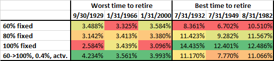
A small caveat, though; the calculations raise the question: do we get something for free? Is this some sort of a money-making arbitrage machine? Of course not! A glidepath will deliver a higher safe withdrawal rate if you have an equity drawdown early on in retirement. But the opposite is true as well. That 60 to 100% glidepath that performed so well during the major Sequence of Return Risk disasters will also underperform if stocks rally during the first few years of retirement. Let’s look at the table below that displays the SWRs of the 60%, 80% and 100% static equity weight and the 60 to 100% glidepath with a 0.4% monthly slope conditional on equity performance. As we already know, it beats the static equity allocation rules significantly when retiring at the market peaks (=worst time to retire). But the glidepath also falls significantly behind the 100% equity allocation if you were to retire at one of the three market bottoms (=best time to retire). It handily beats the constant 60% allocation and is slightly inferior to the 80% constant equity allocation. But I wouldn’t really care too much about falling behind in that case. You still get phenomenal SWR, just a little bit worse than the even more phenomenal SWRs of the 100% equity allocation.
Conclusion
Early retirees need the power of equity expected returns to make the nest egg last for many decades. Even more so than the traditional retiree at age 65! But that exposes us to Sequence of Return Risk. An equity glidepath can alleviate some of the negative effects of Sequence of Return Risk. But it shouldn’t come as a surprise that you will never completely eliminate the risk. For a given withdrawal rate, say 3.5%, we can only reduce the failure rate while leaving some residual risk. And likewise, the 4% rule would still not be safe for today’s early retirees even with an equity glidepath.
Moreover, an equity glidepath is like an insurance policy. A hedge against a tail event! On average it will cost you money, but if and when you need it the most it will likely pay off. Exactly when the static stock/bond allocation paths had their worst sustainable safe withdrawal rates you get slightly better results but you also give up some of the upside if the equity market “decides” to rally some more right after your retirement. But that’s a good problem to have!
Do you have a rule for when we can “reset” our withdrawal rate if our portfolio grows so much that the withdrawal rate is too small?
I would assume that as long as we reset to a rate that has a 0% failure rate it should be fine, but is there a rule of thumb/method that you suggest for handling this?
I don’t have a hard rule. At least once a year, you’d want to re-run the SWR and walk up the withdrawal amounts if desired.
Another approach would be Guyton-Klinger (https://earlyretirementnow.com/2017/02/08/the-ultimate-guide-to-safe-withdrawal-rates-part-9-guyton-klinger/) where you walk up your withdrawals if the current effective withdrawal rate is less than 0.8-times the initial.
What do you think of Kitces rule of increasing withdrawals by 10% for every 50% increase in portfolio?
That seems way too low. If the portfolio increases by that much you can likely increase your withdrawals by 25%+ in the context of CAPE rule. In other words, your withdrawals go up a little bit less 1-for-1 with the portfolio because equity valuations likely also worsened.
Unfortunately, I couldn’t replicate the results with simulation tools like cFIREsim. I had to use passive glidepath since the simulation tool does not support the active method.
Input:
Portfolio: $1M
Withdraw Method: $40K/yr Inflation Adjusted (aka 4% Rule)
Timeline: 55 Years
Output:
80% Fixed: 87.76% Success Rate
100% Fixed: 91.84% Success Rate
60>100%, 0.3%, Passive: 88.78% Success Rate
When using CAPE based dynamic withdrawal method, I got similar results. 94% success with 100% equity while 60>100% glidepath got 91% success rate. But the spending is less volatile with the glidepath.
It’s a great article but I think it suffers from a case of over analyzing/optimization. Even in your table the difference between 80% Fixed vs 60>100% glidepath is small. Though it doesn’t hurt to try since early retirees can rebalance their tax advantaged accounts without incurring income tax.
In my simulations I did not report success rates of the 4% rule, but only fail-safe withdrawal rates. The fail-safe goes up with the glidepath. That’s a very different experiment than looking at the success rate of one specific WR=4%. Also, cFIREsim is only annual frequency. You’ll miss the 9/1929 event. So use the results from that other, inferior tool with extreme caution.
The GP improvement is not small, as you allege. 3.25% to 3.47% is a 6.8% increase in the annual budget. That’s large.
So, in summary, my post is not over-analyzing. It’s exactly the right level of analysis. Your comparisons and allegations lack careful analysis.
Theoretically a higher minimum SWR from your comparisons should yield a higher success rate for other withdraw methods (4%, CAPE, VPW, etc.). Otherwise, it’s too rigid since everyone’s FIRE plan will be slightly different.
For a 5% failure rate with CAPE>20, the difference between 80% Fixed and 60>100% Active glidepath is 3.47% vs 3.63%. To fully take advantage of the active glidepath the retiree would have to actively rebalance every month for up to 13 years. Otherwise, if they do it only once every 6 months or 1 year then they might “miss the 9/1929 event.” Realistically how many people would rebalance so often?
I guess some readers would find value in micromanaging their portfolio on a monthly basis to gain a little bit of a theoretical advantage.
No, it doesn’t. The two objective functions, a) maximize the failsafe and b) maximize the success rate of a specific, WR are not the same. Neither in theory nor in practice. For high enough WRs, it’s best to throw a Hail Mary pass and go all in, hence the better success rates of 100% equities. To maximize the fail-safe rate, you’d want diversification.
Absolutely awesome read, love all your work.
How do you perform this analysis? if it’s done programmatically (such as via python with a stock querying API) could you provide this? I’d love to play with it myself!
For the simpler simulations, i.e., with fixed allocation across time you can use the free Google sheet, see Part 28. But you can do a case study with a Glidepath in that sheet, just not loop over all cohorts with a glidepath.
The Glidepath simulations in Part 19 and 20 were done with Matlab. I will not share the code at this point.
Have you tried using total bond market returns instead of just treasuries to see if that resulted in a higher SWR?
Yes. It doesn’t. The yield is higher, but the diversification is less useful. It’s a wash.
I’m a big fan of your articles Karsten / ERN and have read many of them. I just haven’t had much time to post comments on them.
Anyway I summarized this article to my Dad verbally today, and he and I were wondering what I felt was a reasonable question: can the glide-paths be improved (in terms of fail-safe SWR or failure rate) by only withdrawing from the bond portion of the portfolio if the portfolio is “underwater” (using the same definition for “underwater” as for the active strategy) and the bond allocation hasn’t yet reached its target? Intuitively withdrawing from bonds only when underwater should be a bit more in the spirit of the using bonds as a hedge against equity declines and taking the active strategy a bit further.
I showed that an “active” glidepath can improve results very slightly. But don’t believe that with any kind of scheme to shift the asset weights over time you’ll consistently beat the GP. It’s a hit or miss proposition.
Have you ever run the analysis for this type of glidepath with a shorter time horizon say 30 or 40 years instead of 60 years? I would think that there would be a similar but less pronounced benefit, however, that is just my intuition.
I simulated that in Part 20.
Thanks, I should have just kept reading :).
Dear ERN,
First off, I’d like to thank you for your amazing service to the community! I found your blog a week ago while browsing googling some ideas (the usual) and was flabbergasted at the level of detail, correctness and minutia I found. No half-assing, no misleading presentations, lots of transparency to make the experiments reproducible. In short, a fellow man of ~culture~ science!
I’ve read close to half of your blog entries by now and I haven’t (yet) found an answer to this question, so if you’ll permit (and have the time to reply), I’d love to run this by you:
– How would you approach a situation where someone recently acquired a substantial net worth (e.g. inheritance, sold a business, very quickly accumulated capital) but has yet to deploy it in the market? Lets not complicate and assume no debt, paid off house/mortgage, car/toys/etc and focus on the liquid assets. Considering the extremely high CAPE ratios (~36-37) and a 60y retirement horizon as well as not wanting to deplete the initial value, would you:
a) Glide all the way to 100% stocks over a 10 year period?
b) Set aside a portion of the portfolio to fixed income (e.g. enough real estate yielding 5-6%/yr to cover the cost of life) and dump the remaining assets into stocks on a 60% lump sum + glide path to 100% over 10 years?
c) Same as above but DCA the entire stock allocation into the market over 5 years since the fixed income part easily covers the cost of living (see below) so SRR won’t affect this bit?
d) Some other alternative?
Additional context: I think this might be missing to provide a decent answer so lets also assume a $2M portfolio size and monthly expenses of $60-72/yr. Would this be a moot point since these are below the 3.5% SWR (and because at such a young age finding supplemental income is easy and even a low income value would cover a large portion of the cost of living)?
PS: This might be an interesting blog post. Feel free to use this as a basis if you want and hit me up if you want to collaborate with a data scientist with some OCD ahahah
I’ve written about windfall investing with DCA vs. lump sum here: https://earlyretirementnow.com/2017/05/10/lump-sum-vs-dollar-cost-averaging/
For modest amounts it’s often totally OK to do lump sum, i.e., put in your entire annual 401k limit in January. The longer you’re in the market the better your return, of course. You also still average over many years of your career, so if the market works against you in one year, you still don’t feel too much regret.
For once-in-a-lifetime sums there is the tricky issue of regret. I wouldn’t blame you if you did DCA in that case. So, imagine you want to do the 60/40 to 100/0 glidepath as proposed in my blog post. But you now have 100% T-bills. Do you ant to move $1.2m into stocks and $0.8m into 10Y bonds all at once? Maybe glide into that over a few months to avoid beating yourself up over the exact timing. But I wouldn’t glide from 100% T-bills to 60/40 over 10 years. That’s way too long and that’s not what I wanted to convey with my post here in Part 19 (and part 20).
Dear ERN,
First of all, thank you for the quick and thoughtful reply!
I do understand where you’re coming from (time in the market and expected higher returns in 10-20-30 years from now). I was, however, not expecting you to suggest such a quick entry into the 60/40 initial portfolio. Well, that’s wrong… Let me rephrase that: I was not expecting that suggestion *in light of the currently sky-high CAPE ratios in excess of 35.*
I’ve read the literature (and Vanguard’s whitepaper on it), which suggests LS outperforms DCA 2/3 of the time, but what I noticed in their own fine print is that when there are downturns (and 35+ CAPE ratios do favour a less than stellar forward looking return, even if they don’t necessarily predict a recession), the average outperformance of LS is generally half that of the underperformance. In other words, when things go south for LS, they go _more wrong_ than when they go well. Considering the heightened risks current valuations present, wouldn’t a longer DCA over 3-5 years be reasonable? Looking at prior down markets (1929, 2000, 2008), it would have been pretty effective while not losing a great deal of positive returns.
Perhaps this sounds overly conservative but remember that we’re talking about a life changing amount we’re unlikely to replicate and regret minimization would be the key, since we can probably live off the current nest egg at a 3-3.25% SWR, even with super high CAPE ratios (as shown on your earlier posts), correct?
In other words, we’re trying to assure long-term success and potential for growth, but keeping a (as close to) 100% change of not losing this “golden egg”. What are your thoughts on this? 🙂
A 60/40 portfolio is well-diversified and will sustain your expenses of $60k-$72k p.a. out of a $2m portfolio. So, going into a 60/40 is not the problem except for the “regret factor” I described. Hence my suggestion to spread out the investment over a few months.
But you’re right: I just confirmed that in historical simulations, a glidepath from 100% T-bills to 100% equities would have done even better around the worst-case scenarios (1929 and 1968), so I have some sympathy for your suggestion. If that’s what you’re comfortable with, go ahead. Especially with today’s improved interest rate landscape.
Thank you very much for the peace of mind. Funny how a little validation works wonders!
For what it’s worth, my biggest mistake was thinking the market was overvalued in 2018 and missing the boat to invest regularly since then. I won’t make the same mistake, but CAPE at 36 should give anyone pause when investing such a large sum (IMHO).
Since I already have a portion of my assets invested into local real estate that generate a steady income from rents and renovations, and a solid emergency fund at the short term eur rate, my plan is to be a bit more aggressive than 60/40 by investing the remaining funds 100% into equities – US growth and large cap value, US small cap value, and some EM small cap value.
I just don’t trust the European economy (or China) to deliver risk-adjusted returns in excess of the US (mostly due to current demographics, as well as political and regulatory issues that stifle competitiveness), so I’d rather use real estate to sustain my lifestyle while I wait for the equities portion to grow over the next 10-20 years.
Yeah, trying to time the market like that is hard. The cost of not investing for a while is the FOMO if the market goes up. That’s why DCA is often recommended.
Why separate that out? Growth plus value is the overall blended market again.
I agree with that. I’m not very optimistic about the EU and China these days. US stocks and real estate seem a good bet.
I swore I’d replied to this comment a while ago.. Sorry!
In short, Fama-French. I’m specifically buying large cap with some bias into tech because people will want to keep consuming, even if demographics probably won’t support it in the future. In my opinion, this means productivity/tech will have to pick up the slack to enable growth.
I’d say I view tech as sort of the representation of the human drive to improve and adapt. Then I also focus a bit into the small cap value part of the market to balance out those two factors.
Real estate fills in the developed markets share while also being a more stable income source to avoid touching the equity portion during down markets (and having lots of tax freebies/efficiencies in my country).
It’s not dissimilar to Ben Felix’s factor portfolio, but with some bias towards tech and “hedging” against Europe’s lack of drive/direction.
Sounds like a good plan. Though I’ve never heard of Ben Felix’s factor portfolio.
Hi ERN —
I’m a soon-to-be retiree at the ripe age of 38. I’m currently evaluating the mechanics of starting an equity glidepath, which will involve a hefty rebalancing from a 80/20 portfolio to a 60/40 one. I don’t think I have the stomach to glide all the way to 100% equities, but 85 or 90% seems reasonable. I need something to rebalance with, after all.
To do this in my taxable accounts will make me eat quite a bit in long term capital gains, which I’m not thrilled about. I’ve seen it suggested that I can just buy the bonds in my tax-deferred accounts and keep my sweet, sweet stocks where they are. However, this doesn’t make sense to me, since a bear market would force me to sell equities when they are cheapest, since I can’t actually access the tax-deferred money yet without penalty. I realize I could sell bonds and re-buy those equities in the tax-deferred account, but that still doesn’t feel right, and I worry I’d risk running out of money I can actually use before 59.5.
Do you have any opinions about the actual mechanics of getting into a glidepath vis-a-vis taxes?
Thanks!
Yes, you’d sell equities when they are down, but buy them back in the tax-deferred account. I don’t see a problem with that approach. Money is fungible.
Have you considered making a spreadsheet that allows you to input an after-tax withdrawal rate instead of pre-tax for people who have a lot of money in taxable accounts?
I noticed that as I get farther into retirement, more of the stocks I would have to sell to fund my withdrawal would have higher built-in capital gains I would have to pay taxes on.
So by using a constant pre-tax withdrawal rate, the after tax income isn’t consistent for the entire retirement period.
I tried making a sheet on my own that would withdraw using an inflation-adjusted after-tax SWR, that would make withdrawals from dividends and coupon payments first before selling assets and would keep track of the cost basis of the investments over time.
It was all just too complicated. Do you have a sheet like this or know of a tool that can do this?
No I haven’t because the tax situation is too complex and idiosyncratic.
I’d assign a reasonable average tax rate in retirement and then then gross up your net withdrawals via W_gross = W_net/(1-tax).
You convinced me to start with 60/40. For the bond portion, I was planning to build a tips ladder and also hold vgit. However running the linked monte Carlo SRR model, VWINX Vanguard Wellesley Income Fund seems to good to be true for beating SRR. What am I missing? https://www.portfoliovisualizer.com/monte-carlo-simulation?s=y&sl=6UOyrmWBnglPzl372UPi6O
Portfolio-visualizer “conveniently” ignores all worst-case-scenario cohorts (returns from 1971 onward)
Karsten this is a phenomenal read, so many fascinating insights once I ‘graduated’ from 4% rule grade school! Hope you and your family are having the best early retirement. Off to read the next post.. I could be here a while!! 🙂
Thanks Ellen! Glad you found this useful! 🙂
Do you still recommend using a glidepath strategy for people who have their investments in taxable accounts? I was debating over using a glidepath vs static allocation.
Assuming that someone is in the highest bracket for capital gains and has a long/early retirement (50+ years that the money needs to last), which do you think is better?
I can’t make universal recommendations, but it sounds like if you have only taxable accounts and no way to rebalance tax-free, you still benefit from a GP. You will likely liquidate your bond fund early in retirement (which have little capital gains) and then let the equity gains run. Then liquidate the lots with the highest cost basis first.
What do you think about using a tips ladder instead of a glidepath for the same number of years that the glidepaths in the article above would last?
Would this improve SWR?
See part 61. A TIPS ladder has the same flavor as a GP. Could be a hit or miss. I still prefer the GP. It’s easier to implement for most retail investors.
Is there any benefit to using one over the other if I have almost all of my assets in taxable accounts in the highest tax bracket?
Which method would you say has higher tax drag?
What are the differences between TIPS taxation nominal bonds taxation (as used in my GP simulations)? I’m not a tax expert.
The coupon payments on TIPS are taxed the same as normal coupons (as ordinary income)
The principal adjustment for inflation is taxed as ordinary income every year when the adjustment is made. So you have a “phantom income” each year on that amount even if the bond hasn’t matured yet.
Thanks for confirming! That’s a bit of a raw deal that you pay taxes on the “phantom income.”
Modeling this approach on https://saferetirementspending.com/ did in fact provide an additional 1% to 3% in annual consumption vs using a vanilla glidepath over the same period of time. Using iShares iBonds target ETFs make implementation considerably easier while maintaining flexibility to sell before maturity if needed.
For my analysis I used ladder yields provided by the iShares iBonds target ETFs, matching fixed annual mortgage payments with iShares iBonds Treasury ETFs and other covering most of one’s annual spending with iShares iBonds TIPS ETFs. From there I determined the principal required to fund the iShares iBonds target ETFs ladders and subtracted that amount from the starting bond principle, adjusting the initial portfolio total and initial asset percentages accordingly. If these bond ETFs are held in a tax advantaged account there is no tax drag from the bond ladders. I would be happy to share both export files. Extra percentage of annual consumption below.
Failure Rate Your Filters No Filters Year ≥ 1926 CAPE ≤ 20 CAPE ≥ 20 CAPE ≥ 20; Drawdown = 0%
0.0% 3.27% 3.27% 1.41% 2.81% 3.27% 3.27%
1.0% 2.44% 2.44% 2.41% 2.89% 2.02% 2.62%
2.0% 2.53% 2.53% 2.08% 2.40% 2.18% 2.16%
5.0% 1.88% 1.88% 1.43% 2.94% 2.59% 2.19%
10.0% 1.58% 1.58% 0.71% 3.63% 2.25% 2.18%
25.0% 1.86% 1.86% 0.57% 0.54% 0.84% 2.16%
50.0% 0.56% 0.56% 1.63% -0.22% -1.52% 0.32%
Thanks for doing this. I can’t verify other folks’ simulations.
Why would you hold a mortgage and then hedge the mortgage payments with bond ETFs? Seems more efficient to pay off the mortgage, no?
I have a few reasons for not paying off the mortgage:
1) I am prioritizing Roth conversions for my available ACA constrained tax space. Selling funds from my taxable account would incur large capital gains; pushing me into a much higher bracket, losing all ACA subsidies for a year, and erode much of my taxable account before I could start living off my Roth ladder – adding an extra 10% tax on my early withdrawals.
2) My mortgage has a 2.5% APR interest rate while the bonds in my ladder pay a 1-1.5% higher interest rate.
Noted! That makes perfect sense. With a mortgage rate that low, it’s best to keep that positive carry trade going!
Karsten, Thanks for helping me convince my wife that I could FIRE successfully! I’m starting my 60/40 glidepath to 100 and I’m a bit unclear on the exact logistics.
If I decide to put the extra effort into an active glidepath, how do I decide if the market is at an ATH? Am I looking at an arbitrary but consistent date? I.e. I look at the closing price on the last business day of the month and, if at an ATH convert by 0.4% ? From your chart I would gain a massive 0.05% but, since I like pretending to do SOMETHING, it will be fun. Plus it would be an extra 2k a year for me to use as mad money for my efforts.
https://imgur.com/gallery/active-vs-passive-glidepath-MCq1e98 Failsafe 3.42 vs 3.47
Another question that was asked is “Is it an All Time High or ATH adjusted for inflation?” I posited that inflation was “baked in the cake,” but would love your confirmation.
Well, 3.47 vs 3.42 is a 1.5% increase in the budget. Nothing to sneeze at!
Yes, the all-time high is the total return, adjusted for CPI inflation. Last closing date of the month.
An even better way to massage 0.05%! 0.05%/3.42% = 1.46%
Thanks for making my early retirement less stressful and more interesting 🙂
Yesss! You’re preaching to the choir here, of course. I always note that percentage points are mileading. As you show, 0.05 percentage points can be 1.5% of your retirement budget. Hey, every dollar matters!
Indeed! Just went for lunch and a matinee movie with a bunch of old people (we were by FAR the youngest) and spent some of that 1.5% !
One last question: Do you re-balance every month to make your “new” ratio correct? In my case, in my 1st month of retirement, I started at 60:40 but by the end of the month, because stocks did better, I’m at 60.87 % equities. Market is NOT at an ATH (close buy not quite) so I should be at buying stock to increase to 60.4. Seems simple but I’m at a loss.
Apologies for my laziness: You already addressed this exact issue in detail in part 39. Thanks!
https://earlyretirementnow.com/2020/08/05/rebalance-swr-series-part-39/
Great! Glad you found it! 🙂
For full disclosure: I am not even using the GP myself. There is little rebalancing in my personal portfolio. The GP (Parts 19,20) and the rebalancing study (Part 39) are mostly an academic study for me. 🙂
That’s awesome! “Do as I say not as I do!” It’s why the mechanic has broken down vehicles in his yard, the landscaper’s yard is full of weeds, and the doctor is out of shape while he tells his patient to “eat better and exercise!”
Well, if you ever need to hire a criminal defense attorney, I hope that person has no personal experience either. One can indeed give investing advice about glidepaths to other investors, even if my personal situation doesn’t exactly necessitate it.
Sorry, Karsten. That was poorly phrased with bad examples. I’m sure you didn’t like being compared to a fat doctor.
You’re the expert at this and what you’re advising is for the non-experts. What you can do or should do is on a different level. Here’s a better example of do what I say not what I do: I advise people to get colonoscopies to diagnose and treat colon cancer early. Personally, I’m never getting one! The “NNT” (number needed to treat) is too high for my tastes. You have to stick a snake up someone’s butt 1,013 times to prevent ONE death. Do you diagnose others earlier? Sure! Is there life better? Not so sure. I don’t want to spend one day pooping on the toilet and another doped up on the less than 1:1000 chance it’s going to save my life.
It’s not general advice but informed by expert opinion and data. Pretty sure you don’t need to do a glidepath (or have decided you are taking an acceptable risk), but thanks for pointing out the option to us average investors :-).
Correct. That was my intention: Give people options. Let folks decide if they believe the small increase in the SWR is worth the effort. 🙂
Big ERN,
Thanks for my favorite finance blog! I’ve been approximating the glidepaths in your spreadsheet by simplifying the strategy:
A) Put 6 years of expenses into a cash account (or CD ladder)
B) The remaining nest egg is kept in 90/10 stocks/bonds, rebalanced as needed.
In retirement, pull from A until it’s depleted in 6 years. Never refill it; just switch over to B. A’s gradual depletion creates a natural and simple glidepath similar to what’s in the post.
Results match your more in-depth simulations with reasonable accuracy. Does this approach seem reasonable? Easier? Worse?
That’s a totally fine approach. Most of these glidepaths are very similar in spirit. I’m not surprised if your results are similar to mine.
I just want to say thanks for putting together such a great website. I wish I found it decades ago, or a decade ago, or even 5 years ago… There is so much garbage in the FIRE blogosphere by people trying desperately to generate income because they “retired” with too little. They waste so many electrons simply saying “cut spending” and “withdraw 4%” hundreds of different ways, telling readers what they want to hear. But not this site! This site looks at the math and data and isn’t afraid to suggest that early retirees consider less than 4%!
Thanks for the words of confidence!
But I also often recommend more than 4% if the supplmental cash flows and/or market conditions allow. See Part 54.
Sorry is there a new spreadsheet recently available from Big ERN that we can actually calculate the rising equity glidepath?
No. You can use the spreadsheet and simulate a rising GP for one specific cohort but not for all cohorts. I had to run these sims with Matlab over a large loop.
Sorry is that just being done on the Parameters & Main Results tab by adjusting the portfolio mix and retirement horizon to see how the WR/SCR change?
Tab: “Case Study”
Enter the GP parameters in G10 to H22.
Got it, one more question please. Any insight into what year for the retirement start to look at this through a “conservative” lense?
Usually, 9/1929 & 12/1968 are the historical worst-case cohorts. 🙂
Thanks. Just confirm the “end of month portfolio value” at the end of the simulation is the Real value (the value in today’s dollars)?
Correct. Everything is real value: the withdrawals are also adjusted to CPI and the final portfolio value, too.
Hi Dr. Jeske, this is a great post! In my own analysis, I also found that equity glidepaths were effective. One question I have for you is around the tax implications of the glidepath. In the accumulation phase, one can freely sell and rebalance within tax-advantaged accounts such as (traditional) 401k and Roth IRA. However, rebalancing a brokerage account will have tax implications (due to capital gains).
Similarly, post-retirement rebalancing would incur similar penalties. One idea that I had was to simply rebalance the 401k and Roth IRA to be bond-heavy enough to have an _overall_ portfolio that matches the desired starting point for the glidepath. However, some criticisms of that approach include the fact that it feels like it’s an unoptimal use of tax-advantaged space.
Another idea I had was to instead go heavy on investing in bond index ETFs and leave stock index ETFs by the wayside during the final years of the accumulation phase, thereby altering the taxable brokerage account’s ratio towards the glidepath starting point. Of course, the tax-advantaged accounts could be freely rebalanced whenever without concern. This would imply that each account’s fund ratio represents the overall ratio (a “similar triangles” kind of approach).
Do you prefer the first approach or the second? Or do you just simply sell and accept the 15% LTCG tax to achieve the rebalancing (I assume almost certainly not).
Thank you for your time. I hope retirement is treating you and your family well!
You rebalance in the tax-advantaged accounts. Both during the last years of accumulation to build up the bond tent and also during the reverse GP in retirement. If your tax-advantaged accounts are large enough, e.g., greater than 40% of your portfolio there should be no issue keeping all equities in your taxable accounts and letting the tax-advantaged accounts do all the rebalancing.
Hi Dr. Jeske, that makes a lot of sense! And I guess when withdrawing during retirement there is also a natural rebalance by taking out bonds first to slowly glide towards equity-heavy in deeper retirement.
Thanks for your reply!
Thank you for all of your research. As a new early retiree, it’s all been incredibly helpful.
I started rebalancing to an equity glidepath using the active approach, and while building out my path, I started thinking about a hybrid passive-active approach, and wondered how you think it would perform relative to the active approach.
In this hybrid approach, the target equity percentage increases monthly no matter what (passive), but you only rebalance to that target when equities are below the all-time high (active). The total transition time would be the same as the passive model, but like the active model, you would only be shifting more into equities when they are below highs.
For example, say we are actively gliding from 60% to 80% at 0.3% per month. We are currently at 63%, so the next shift will be to 63.3%. However, the S&P500 is within 1% of the 52-week high and stays there for 3 months. At 3 months, there is a dip, and we can resume the transition and rebalance.
With the active approach, we pause at 63% equities for 3 months, and when the market dips, we rebalance to 63.3%.
With the hybrid approach, we also pause at 63% equities for 3 months, and hen the market dips, we rebalance to 63.9%. (While pausing, the target continues to grow 63.0 -> 63.3 -> 63.6 -> 63.9).
Sounds like a great plan. I don’t think that the details matter that much, as long as you shift up the weight. The exact implementation has a small effect on the final outcome.
Agree with ERN here, but it’s funny that this approach is what I always thought the active approach would be (/facepalm). Otherwise, the active path would take far longer than the drift (0.3 or 0.4%) would imply, no?
For example: 40->100 0.4% GP: (100-40)/(0.4*12)=60/4.8=12.5 years to complete the glidepath. With pauses at ATHs, it’d probably take closer to 15 years, no? Not sure I’d be comfortable with such a long GP, even being stupidly conservative as I am.
PS: For the record, I’m completing a 3 year GP to 60% of my target equities allocation before I transition to a 60-100/.4% active as well (business took off and then sold it is how I ended up with such a low equity allocation, before you judge me insane ahha).
PPS: I say 60% of my target equities allocation because my portfolio is 70% equities and 25-30% in real estate I don’t plan on selling (stable cashflow for discretionary spending optionality on SORR materialization). I’ll drift to 60% of those 70% by end of 2026 and then glide to 100% of it (70% of the portfolio) in the following 6-8 years (not 8.3 because I assume there’ll be a crash that’ll accelerate my buy-in).
Hope this helps and would love thoughts from both of you!
12-15 years of GP is actually what you want. It should be a market cycle or even two.
You’re saying that for a 0->100% GP you’d do a 12-15 years GP? Did I get that right or am I missing something?
I’m confused because on the SWR series entry on GPs (#2, I think), the GPs starting off from 0 performed horrendously, didn’t they? I thought the ideal was a 40 (or 60%) to 100% GP for optimal SWR?!
Would you be so kind as to clarify, please? 🙂 I thought I was being conservative in doing 0->60 in 3 years and then 60->100 in 6 to 8! Now I’m scared ahah
Sorry, must have misunderstood the question. 60/40 to 100/0 would take that long. 0/100 to 100/0 would take way too long. I would not start with 100% bonds.
Fair point. Currently at 20% equities, 60% short term rate ETFs and 20% real estate (recent large cash infusion). Plan to make it 40% (60% of final target allocation) in equities by end of next year and then a 0.4% GP to 70% (100% of final allocation).
Makes sense or would you do it differently? I think this fits well with what you showed would be optimal for glidepaths and equity allocations, especially considering current valuations. Real estate is just a SORR mitigator, as it guarantees I don’t have to touch the equities portion during a downturn in the first 5-10 years of retirement.
I know RE lowers total expected returns over the long run, but the downside protection is worth it IMO, now I’m pretty close to the number I want.
Yes, that makes sense.
Also, depending on what exact RE investments you have, I wouldn’t discard it as lower returns. Some RE investments will have great returns, as I see with some of my private equity (multi-family) RE returns so far. So, no worries there.
Awesome. That takes a load off my back. As usual, thank you Dr Jeske! 🙂
You bet! Good luck!
While playing with your online calculator, saferetirementspending.com, I noticed that the 40 to 100 glidepath loses to the static 80/20 allocation if the Final Value is more than 33% over the 30 year retirement. To determine who “loses” I compare Failsafe for CAPE>20. The difference increases with the Final Value, and becomes quite substantial at 50%. I am somewhat puzzled by this result because intuitively the glidepath should win.
How long did you set the GP? The entire 30 years? If the GP is too slow, it becomes counter-productive.
I tried two GP lengths: the 100 month default and then 120 months, which I think is what you did in the post. The former did better but either one was worse than the 80/20 static. When I switch to the Final Value zero, the GP wins.
Apparently, the 40/60 starts too low. Have you tried 60/40 to 100/0?
After some trial and error I found that for my specific cashflows and the Final Value an optimal strategy is the 15 year glidepath from 15/85 to 90/10, which beat the static 70/30 by 4% of annual consumption subject to CAPE>20 constraint. I feel uneasy starting the glidepath at the 15% equity. I am worried about missing the upside if the bear market does not materialize. In any case, my point still stands: the Final Value has a significant impact on what strategy is optimal and GP does not always win.
Well, that’s the cost of insurance. That’s why I kept my equity exposure at around 70% all through my retirement. Helps with FOMO when the market keeps rallying.
With Cape 10 being just under 40 as I type this, is it advisable to hold the starting asset allocation (say 60/40) while markets are high and then start the glidepath when a correction hits? Conversely this seems like market timing given the run on equities could continue for a while longer and one would miss out on some of those gains. I didn’t see this addressed and apologize if it was already.
I think the answer is an “active” glidepath. You only move when the market is NOT at an all time high (adjusted for inflation). I hadn’t thought about it as market timing, but I guess, in a very small way it is. If you study Karsten’s charts closely there is a small benefit to the active version. In my case it was 0.05% increase in the safe withdrawal rate. But, with the magic of fractions and decimals, that becomes a 1.46% increase in cash flow :-).
I agree that the active glidepath as described is not really market timing. However I was referring to waiting for something like a correction (a 10% drop) before starting the glidepath which could take a while.
That’s exactly the definition of the active glidepath.
Thanks! Couldn’t have answered it better!
Nick Sartor answered this well!
How much tax drag do you think the 60 to 100 .3% passive glidepath would have if my entire portfolio was in taxable in the top bracket?
Do you have a spreadsheet for this?
I don’t have a spreadsheet for that. It may not make a big difference because you might simply leave the stock portfolio untouched and liquidate the bond portfolio over 10 years. Since bonds don’t have as much potential for large capital gains (certainly less than NVDA, haha) you may not get hit by capital gains taxes, even if all your asset are in a taxable account.
I tried doing glidepath SWR calculations using your 3 month bond return data from your toolbox instead of 10 year bonds and it gave me higher SWR’s.
Is this consistent with what you find or did i do something wrong?
For more information i did an ititial 60% stock, 40% short term (3 month) bond allocation with a .3% monthly shift towards 100% stock allocation and it gave me an SWR of 3.6% which is higher than the 3.44% shown above using 10 year bonds.
It’s possible that your current failsafe falls into the 1970s era, so you would have done better with low-duration for your diversifying asset. So, yes, that’s absolutely possible. But the opposite is also possible if your failsafe is the Great Depression.
How would SWR change if i wanted to use a total world stock index instead of sp500?Assuming that i still use a 60/40 to 100/0 glidepath and i am in taxable accounts.
You can simulate that in the SWR toolbox. I have the data for MSCI World-ex-USA since 1970. Use 0.50 USA and 0.50 non-US and you’d likely see a slight improvement because there was some nice diversification, not so much during the recessions and bear markets but during the recoveries.
Then again, non-USA performed quite poorly post-2009.
Hello ERN! I’ve been reading your blog the past few days and loving it. It seems your math leads to the conclusion that rising glidepaths with a stock/bond portfolio are best. I have doubts about the glidepath method I wanted to ask you about.
Keep in mind I’m new to this and what I’m writing is based on personal sentiment. Definitely not the sort of rigourous analysis you present with every post, so I’m sorry if it’s nonsense (also english is not my first language).
My doubts and what they’re driven by:
– Positive correlation between stocks and bond returns (as seen in recent years)
Are bonds really a good hedge? There are many points in history where bonds have a positive correlation with stocks, and in my understanding, it unfortunately happens most often when both are falling.
Wouldn’t cash be a more stable, less volatile option? Are there any others?
– High capital gains tax (no tax advantaged accounts)
Is frequent rebalancing a good idea in this case? Wouldn’t it be better to simply dip into the non-stock asset when the market is down?
Also since the high capital gains tax makes me a bit reluctant to sell a big portion of my stocks, I’d have to build my bond allocation with steady contributions throughout the years, losing me the nice juicy stock returns. If during the retirement glidepath bonds and stocks also start falling in unison, that would be awful hahaha.
– Long stagnant market followed by a market crash
Sideways returns for that long are probably not likely if I’m globally diversified, but considering the high taxes and the fact that bonds don’t generate much surplus capital, I think it would be better for me to liquidate more of my bonds early in retirement (making my glidepath quicker).
I don’t know how likely this is, but I wouldn’t want to complete my glidepath during a sideways market, and then have a stock market crash right after I’m done with my reallocation to 100% stocks. Again, wouldn’t using the non-stock asset only during market downturns solve this?
With these considerations, wouldn’t having 100% stocks + 3 years (long bear market duration) worth of expenses in cash, and then dipping into the cash only when the market is down a certain amount (say 10%), with no replenishing or rebalancing, be a better strategy?
Thank you if you read this, and sorry if the comment is too long. Have a nice day!
Sometimes bonds have a positive correlation (supply shocks), i.e., 1970s and 2022. Most US recessions are demand shocks, though with a zero or even negative correlation. Even in the 1970s, stocks + bonds did better in retirement portfolios than 100% stocks.
Rebalancing: You’re free to not rebalance. The rebalance frequency is not that crucial (see part 39). If you absolutely no tax-advantaged accounts you’re a small minority. Most people can efficiently rebalance.
Long stagnant market plus sharp drop: That would be not ideal for the glidepath. But even in 1968-1982 (long stangant market plus sharp frop in the 70s and 80s) the GP helped (somewhat)
100% stocks + 3Y cash? Now you’re at 85% stocks + 15% cash. So, you do have a (slightly) diversified portfolio. You could do even better with moving from 60/40 to 100/0. You could do even better with at least a part of 10Y Treasury bonds as diversifier.
Have you ever looked at using deep out-of-the-money puts to hedge against black swan events instead of using bonds?
Yes. But it’s expensive. Please see my options writing series on why I believe that writing deep out-of-the-money puts is the way to go for extra income and then then reduce the portfolio’s equity portion. See here: https://earlyretirementnow.com/2025/01/14/options-trading-series-part-13-year-2024-review/ Especially the discussion about Bob Litterman’s video.