A Safe Withdrawal Rate Case Study for Becky and Stephen

What? A new case study? I know, I had promised myself to wind down the Case Study Series I ran in 2017/18 after “only” 10 installments. It was a lot of work and a lot of back and forth via email. It takes forever! I mean F-O-R-E-V-E-R! But then again, there’s always a reason to make an exception to the rule! Jonathan and Brad from the ChooseFI Podcast had a very interesting guest on their show this week (episode 152). Becky talked about her experience of a late start in getting her and her husband’s finances in order. They started at around age 50 and became Financially Independent (FI) in their early 60s and retired a year ago. I should also mention that Becky recently started her own blog, appropriately labeled Started At 50, writing about her path to FI and RE so make sure you check that out, too.

In any case, Jonathan and Brad asked me to look at Becky’s numbers because I must be some sort of an expert on Safe Withdrawal Strategies in the FIRE community. I chatted with Jonathan and Brad about my case study results the other day and this conversation should come out as this week’s Friday Roundup episode. Because there’s only so much time we had on the podcast and I didn’t get to talk about everything I had prepared, I thought I should write up my notes and share them here. Heck, with all of that effort already spent, I might as well make a blog post out of it, right? That’s what we have on the menu for today…

Background

• Becky and Stephen (63 and 64 years old) live in Colorado and retired about a year ago.
• Their current nest egg is about $1,355,000 in financial assets.
• They also own a single-family home, mortgage-free, worth around $450,000 today.
• They are planning to live on around $80,000 after taxes, so they have pre-tax cash-flow needs of close to 90k per year. That would be a 6.6% initial withdrawal rate; sounds really high, but there are special circumstances that will make this withdrawal rate sustainable! More on that later!
• $60,000 of their budget is the non-discretionary base budget. $20k is for fun stuff and that figure can be reduced if necessary.

Social Security/Pensions: [Update 11/9/2019: I recalculated the Social Security timing with the help of “OpenSocialSecurity.com“]

Stephen had very high FICO/payroll taxable salaries throughout his life. He got pretty close to reaching 35 years of contributions at or close to the Social Security annual limit, so he expects $3,500 per month at age 70! Becky’s own benefits at roughly $1,000 are substantially lower than Stephen’s. 

I found a great tool online: opensocialsecurity.com/ to determine the optimal Social Security timing. This is particularly useful in this case when you want to determine the timing of spousal benfits! The inputs: First Becky, who I assume was born in 1956, mid-year. Her own PIA (Primary Insurance Amount), i.e., the amount she’d get at full retirement age is $1,000:

Her husband is one year older and expects $2,680 PIA (which would translate into $3,500 at age 70!). You can also add the mortality table to reflect that they don’t smoke (I presume) and are generally very healthy (“Nonsmoker Super-preferred”)

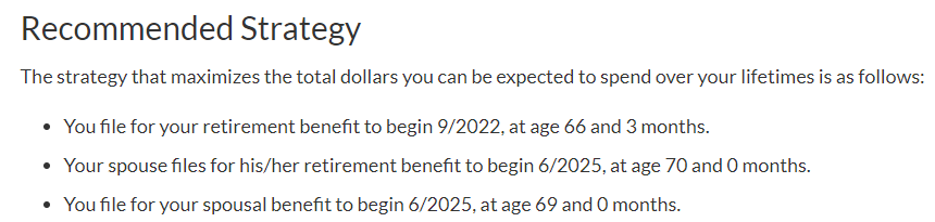
And click “Submit” and the site spits out the recommended Social Security claiming schedule. Becky files for her own modest benefits in 2022. Then Stephen waits as long as possible, until age 70

The approximate benefits per month are (rounded to the closest 10):

• Becky on her own benefits: $990 in month 67 of the simulation (9/2022)
• Becky while on spousal benefits: $1,330 per month (11,933+4,080 annually). Basically, Becky’s benefits will be topped off to match half of Stephen’s PIA. Why this is not exactly equal to 1,340, I can’t tell.
• Stephen: $3,500 when reaching age 70.

Notice that the combined benefits amount to around $58k per year. That means, only six short years into retirement, they can reduce their withdrawals from the portfolio very substantially! 

Other parameters/considerations:

• Around 17 years into retirement they like to scale down their budget by $10,000 p.a. due to less travel and just in general, living at a slower pace. I heard they currently drive vintage Porsches (yes, plural!) and when you reach your 80, it might be time to also literally slow down. Maybe switch to a Toyota Avalon?
• Around 21 years into retirement, account for the possibility that one spouse passes away. Social Security benefits are now “only” $3,500 per month (either Stephen’s benefits, or Becky getting survivor benefits). I assume the expenses stay the same, to be conservative. In reality, some expenses will go down but that’s also likely offset by a less advantageous tax landscape when the survivor has to file taxes as a single. So, my working assumption is always that when a spouse passes away the lower expenses and the higher taxes are a wash.
• Around 25 years into retirement, the surviving spouse will sell the house (value $450k in today’s dollars) and move into an assisted living community. This will raise the annual budget to $150k. Not quite Suze Orman territory but still a very generous budget!
• Becky wants the money to last until age 95-100 and still have $1,000,000 left as a cushion for health costs. I’d think that $150k a year covers a nursing home plus health costs pretty well, though, so I think that $1m figure is a bit of overkill.
• Becky and Stephen have kids and grandkids, but they haven’t explicitly factored in a major inheritance for their heirs. It sounds like they want to be generous while still alive, great idea!!! I also think there will be plenty of money left because a) the nursing home budget seems pretty generous and there is a high likelihood that you don’t live all the way to 98 or 100. So, with a large probability, there should be money left over for the kids/grandkids.

So, it looks like Becky and Stephen’s retirement will go through 3 major phases

1. The first six years of very large withdrawals to fund expenses before Social Security kicks in,
2. The next 19 years of living off Social Security with relatively small cash flow needs from the portfolio,
3. The remaining years start with one large cash inflow. But then we also throw the regular budget out of the window and budget for a very generous $150,000 withdrawals in today’s dollars, which is more than 10% of today’s portfolio!!!

A few preliminary observations:

81.7% in a stock portfolio seems a bit high for retirees who plan not to work on the side. I will later recommend an allocation of 60% Stocks, 35% bonds, 5% Cash/Money Market, which is more appropriate to hedge against Sequence Risk. If you absolutely want to keep your 80+% stock share, it wouldn’t be too catastrophic either, but you’ll add some (unnecessary) risk! Remember, in retirement and in FI, you already won the game, why keep gambling?

Taxable bonds are in the taxable account. That’s inefficient! It crowds out your Roth conversions because the bond interest is ordinary income! Ideally, you hold taxable bonds in a tax-deferred account. Of course, people then wonder how can you withdraw bonds when you have 100% stocks in your taxable portfolio. It’s easy: money is fungible! Imagine you own only stocks in a taxable account and a Roth IRA with stocks and bonds. If you want to withdraw a certain amount from bonds without touching the Roth, simply take that amount from the taxable stock portfolio. But then in the Roth IRA move that same amount from bonds into stocks! Again, money is fungible!

So, I would suggest getting rid of all bonds in the taxable account (and buy bonds in the T-IRA and/or Roth to offset that). If that’s too intrusive for you, at least liquidate the taxable bonds first to finance the living expenses early on. And again: shift money from stocks into bonds in the retirement accounts to compensate!

Setting up the ERN Google Sheet

Let’s get our hands dirty! Here’s the link to the Google Sheet I prepared:

Becky and Stephen Google Sheet

As always, please save your own copy if you want to play around with the numbers. I cannot grant you permission to edit my official Google Sheet because I have to keep a clean copy for everyone! I won’t give you access to my brokerage accounts either! 🙂  To save your own copy, click File/Make a copy, see below!

Parameters in the main sheet:

• Allocation: Stocks 60%, Bonds 35%, Cash 5%. I played around with the asset allocation and the 60% stock allocation had the best-looking fail-safe properties. Sure, with 80+% stocks you will do much better on average, but you’ll also add some tail risk and the potential to run out of money 30 years into retirement!
• Horizon: 35 years = 420 months (Becky 98 years old or Stephen 99 years old)
• Final Value Target = 0% of initial capital. For now, I set this to 0 because I think that with the $150k annual budget for the assisted living/nursing home we’ve covered a lot of medical expenses already. Simply make sure you don’t completely run out of money if you live to age 98+ and leave a large inheritance if you die earlier! We can always look at what’s the historical distribution of the final value and check what are the probabilities of a final value >$1m!

How do we implement the supplemental cash flows from Social Security etc. in the spreadsheet? Let’s take a look at the tab “Cash Flow Assist”  (ignore the part about the CD ladder, we’ll deal with that later!)

• Social Security
  • Becky’s own benefits in month 35: +$990
  • Becky’s own+spousal and Stephen’s benefits in month 68: +$1,330 and +$3,500, respectively.
• 17 years into retirement (month 1+17*12=month 205), when Becky and Stephen are in their mid-80s, they will scale back their expenses by $10,000 per year. This will show up as a positive cash flow of $833/month
• 21 years into retirement (month 1+21*12=month 253), one spouse passes away. Becky’s SS benefits go away.
• 25 years into retirement, sell the house. Let’s assume that the $450k house maintains its value in real terms, i.e., appreciates in line with CPI. But also assume broker and other transaction costs of 8%=$36k. Net proceeds=$414k. The surviving spouse moves into an assisted living facility. This will raise the annual budget from $70k to $150k, so we enter a negative monthly cash flow of $6,667 starting in month 302.
• Taxes: See this post on how Social Security is taxed on the federal return.
  • Until Stephen claims his Social Security: Assume $8,000 p.a.  So, I enter -8,000/12=-666.67 in the first 67 months. 
  • For the next five years, let’s assume taxes are a bit lower because we’re done with the aggressive Roth conversions. $5,000 p.a. (very conservative, likely lower in real-life), so I enter -$416.67 in months 68 to 127
  • After that, your tax liability drops to $3,000 p.a. That is again quite conservative because it’s likely that you will have depleted your taxable savings and rely on Roth contributions plus Social Security (plus a few T-IRA distributions). $3,000 tax liability, again quite conservative, so I enter -$250 in months 128 to the end. Colorado does tax your income with a flat tax of 4.63% income but it has some generous exemptions ($24k per year for 65 years and older). Note: I’m not a tax expert. I’m not a Colorado resident either, so I have to rely on data I found online. I normally use the Kiplinger State-by-State Guide to Taxes on Retirees.

Wow! That’s a mouthful! Let’s summarize the cash flows over time:. The Google Sheet searches for the initial safe consumption amount x (set to $80k in this example). Note that I didn’t display the large cash flow from the home sale which would show up as a “negative withdrawal” but it would blow up the scale! 🙂

A quick technical note: The way I set up this case study is to do the Safe Consumption part for the first 25 years only, so playing around with the initial withdrawal amount x has no impact on the flows after month 301 when the cash flows are predetermined at +3,500 Social Security, $-12,500 for the nursing home and $-417 for taxes. To implement this in the Google Sheet I set the “scaling of withdrawals” to 1 for the first 25 years (months 1 through 300) and to 0 starting in month 301.

And another side note: a common question I get is how I deal with inflation in my calculations. All of the cash flows I’ve mentioned are in 2019 dollars, so in the calculations, I assume that they will go up with inflation. Thus, they are entered in the section labeled “Cash flows that will be adjusted by Inflation (e.g. Social Security, public Pension, etc.): Enter in today’s $”

Detailed results

First of all, forget about the 4% Rule. The initial consumption rate is much higher, closer to 7% and you can afford this in light of the substantial Social Security benefits just around the corner. Here’s the table with the safe withdrawal rates in the main tab of the sheet.  It turns out that the overall worst failsafe was 6.60% (though that would have been pre-1920). After 1926, 6.73% would have been OK, which translates into more than $90k!

I also display the safe rates by market event and by decade (1920s and forward) below:

If you prefer to see these numbers in dollar amounts you can also see the same tables as dollar figures in the tab “Cash Flow Assist,” see the table below:

So, it looks like $80,000 annual consumption (plus the provisions for taxes!) is ironclad and super-safe. And again, this $80k budget is for the first 17  years, scaled down to 70k until year 25 and then $150k for the remainder. But that doesn’t mean it was a smooth ride! Let’s take a look at three prominent bear market scenarios:

• (1/1916: let’s ignore the pre-1929 experience for now. This was the worst experience in a previous version of the case study)
• September 1929 is the market peak right before the Great Depression!
• December 1968 is the cohort worst hit by the tumultuous 1970s and early 80s! If you remember last week’s post, this is one of the worst bear markets in history when measured by how long it took to recover!

The chart below plots the value of the portfolio (adjusted for inflation) of the three disaster cohorts over their 35 years of retirement. Notice how they all survive the 35 years and have about $800 (1916) and all the way up to the desired $1m+ (1929, 1968) as the final value. But it was a rough ride! All three cohorts drop below the $600k mark, two of them even below $500k only to recover again to the seven-figures club, especially after the massive cash inflow in month 300 due to the home sale.

How likely is it that you still have a $1m cash cushion at age 98? In the Google Sheet, I created a tab “Distribution of Final Value” to study the distribution of the final values for the historical cohorts. I sorted the final asset value (expressed as multiples of the initial value) from lowest to highest (though in the chart I go only up to the median = 50th percentile) and plot it in the chart below. So, I can read off, what’s the probability of falling below a certain final value, especially in the left tail of the distribution!

For the math/stats geeks, this chart is essentially the historical “cumulative distribution function (CDF)” but with the axes flipped! 🙂  In any case, historically you would have had a roughly 5% chance of ending up with less than $1m and a 14% chance of ending up with less than the initial portfolio value. It seems like $80k is a pretty solid withdrawal strategy that a) never would have run out of money in past cohorts and b) had a reasonable probability of maintaining the portfolio over time. Though, again, I like to stress that a lot of historical cohorts had massive drawdowns along the way, especially if the market was weak during the first six years!

Recommended withdrawal sequence

The SWR Google Sheet just considers all the different accounts as one single big portfolio. In practice, however, we still have to determine what accounts we like to tap in what order. My recommendation:

• Withdraw the taxable bonds, cash/money market first. This should suffice for about 3 years worth of expenses and taxes. Then liquidate taxable stocks.
• Because you’re withdrawing the taxable assets with a very high tax basis first, you should realize only very minimal taxable income. Use the “space” in the standard deduction plus the 10% federal tax brackets and even a bit of the 12% bracket to do Roth conversions. You should be able to do around $50k every year until Social Security starts. The idea here is that you want to make a meaningful dent in your Traditional IRA. But don’t go completely bonkers with the Roth conversions because we can still withdraw a small amount of the T-IRA tax-free even when Social Security kicks in. Being too aggressive with the conversions would mean that we leave those tax-free IRA withdrawals on the table!
• Also, notice that your annual standard deduction is raised by $1,300 per person above the age of 65! Use that to max out your Roth Conversions!
• Once Social Security kicks in, we have to go through a pretty arcane calculation to figure out how much of those benefits are taxable on your federal return. Initially, I worked under the assumption that it’s 85%. But the calculation is more complicated. It turns out that even with $58k in annual Social Security benefits, the fraction taxed on your federal return is a lot less than the 85% I assumed. We can even hack this so that your T-IRA withdrawals still fall into the standard deduction. See the post on 11/20/2019 about the recommended Roth Conversion strategy.
• Required Minimum Distributions after age 70.5 (the age could potentially be lifted from 70.5 to 72 if the Secure Act passes, see Forbes article here!) shouldn’t be an issue. The RMDs will likely be lower than what you withdraw to fill up your Standard Deduction.

The calculations for how fast or slowly you should convert are a bit too involved to add here to this already very long post. (and by the way, I’m the Safe Withdrawal Rate dude, not a tax expert!!!)  I will write a new post on this Roth conversion conundrum, probably by next week to update everyone!

Also, notice that one of the common challenges of the extremely early retirees doesn’t apply here! Becky and Stephen are past age 59.5 and can tap all of their retirement savings penalty-free (though not tax-free). So, there are none of the cash flow hassles we normally face where you have to make sure you have enough taxable accounts and/or Roth ladders with the 5-year lag between conversion and withdrawals!

By how much can they increase their budget?

After I finished the study and told Becky that it looks like their $80k a year budget is a “go” she asked me if they can up their budget to $90k. Well, we know from the tables above that the failsafe consumption amount was just under $90k. What cohort would have run out of money consuming $90k? You guessed it: 1968. In the chart below I plot the time series for that cohort under an 80k, 85k and 90k annual consumption budget, respectively. It turns out, the 1968 cohort was the one that will not digest the cash flow pattern that Becky and her husband plan very well. You’d have almost run out of money toward the end. More worrisome than that, though is fact that the 1968 cohort would have depleted their portfolio to all the way down about $400k after 25 years. Adding the home sale would have brought you up to a bit over $800k in month 300. It’s only because of the start of a major bull market of the 1990s that you even made it that long with $150k of nursing home expenses per year! So, for me personally, moving into a nursing home with such a small nest egg would not make me very confident and comfortable. Maybe start with $85k and see how that goes for the first few years!

Use a glidepath?

As I pointed out in Part 19 and Part 20 of the SWR Series, one way to alleviate the impact of Sequence Risk is to use a “glidepath,” i.e., start with a lower than long-term sustainable equity weight but then shift back into equities over time. One way to implement this is to shift, say, $300k into a CD ladder. Let’s assume you get around 2.25% nominal interest. Over a 72-month period before Social Security kicks in that would get you about $4,450 per month. So, we reduce the portfolio by $300k to $1,055,000 but we compensate for it by adding the positive nominal cash flow in the Google Sheet, see below.

You now have an initial allocation of 47/27/26 Stocks/Bonds/Cash, only to shift back into the long-term target allocation of 60/35/5 over time once you reach Social Security. Would that have saved the 1968 cohort? You bet! But again, you would have moved into the nursing home in year 26 with an extremely depleted portfolio. Still not a very comforting scenario. But it’s good to see that the glidepath at least alleviates some of the Sequence Risk during the first six years!

Other thoughts

There will be a large cash infusion when you sell the house. I assume it’s $414k in today’s dollars (after 8% transaction costs). What do you do with this large cash infusion? Currently, I assume it goes back into the nest egg (taxable account) at the prevailing 60/35/5 allocation. Sometimes people are too afraid to invest such a large lump-sum, see the discussion on lump-sum investing vs. Dollar-Cost-Averaging (both here on the ERN blog and in my initial ChooseFI appearance, Episode 35). One alternative would have been to build a bond or CD-ladder (see my CD ladder toolkit!) to take the home sale proceeds and fund the first several years of the nursing home with that. That’s certainly feasible and also desirable (it lowers Sequence Risk) but it’s also impossible to forecast the interest rate landscape that far into the future. It’s a battle that’s best fought at that time.

And again, in case I haven’t stressed this enough, be prepared to draw down the portfolio, at least initially. If the market is weak over the first six years and you withdraw 6+% p.a., then you will very likely draw down the portfolio. If the market is really bad you might draw down all the way to $500k!!! But don’t despair! Because your withdrawals will be so low once SS kicks in, you’ll have plenty of time to recover!

Conclusions

As I said on the podcast already, it looks like Becky and Stephen should have a safe and comfortable retirement. They can even raise their budget a little bit. Though, I’d be cautious about going all the way to $90k per year. Maybe start with $85k for a few years and see how things work out.

In any case, I learned a lot from doing this exercise. First, you’re never too old to get your financial act together. All of the principles of FIRE apply here, too. Even at 50 years old you can still shoot for a comfortable retirement in your early 60s, way earlier than most other Americans. I’m so grateful to Jonathan and Brad for bringing Becky on their show because we all benefit from having a more diverse FIRE community. FIRE in general and ChooseFI, in particular, are all great sources of inspiration and information for all age groups!

Second, “older early retirees” (if there’s such a term) have a number of advantages: higher Social Security benefits due to more years paying into the system, less time until benefits start and also less political uncertainty about the size of your benefits. The shorter life expectancy, while obviously nothing to cheer about, is also at least a mathematical advantage over the extremely early retirees. So, the initial consumption rate is much closer to 7% here in this case study! Another example where the Trinity Study and the plain old 4% Rule is of no help. You have to get your hands dirty and make this a customized and personalized safe withdrawal analysis!

I am also encouraged that the prospect of some large future assisted living and nursing home care expenses does not sabotage their comfortable early retirement. Take that, Suze Orman!

Best of luck to Becky and Stephen!

Thanks for stopping by to read today’s post! Looking forward to your comments and suggestions below!