


It’s time for a new post in the Safe Withdrawal Rate Series. It’s been a while, I know! This is a post I’ve been mulling over for a long time and a recent suggestion from a reader made me revisit my notes again. Why not calculate sustainable withdrawal based on how accountants or actuaries work. No simulations necessary! Neither historical nor Monte Carlo simulations! And here’s the kicker: you run this SWR calculation with all the data you’re going to assemble to use my Google SWR Sheet already. No extra work necessary! So, what do we have to do? Very simple:
- Take stock of all of your asset and liabilities today
- Take stock of all of your future expected cash flows: both positive (Social Security, Pensions, etc.) and negative (health expenses, kids’ college expenses, etc.).
This is essentially the information that you’d already need to know when doing a Safe Withdrawal Rate analysis, specifically, the inputs for the Safe Withdrawal Google Sheet, see Part 28 of this series!
So, how do you calculate a safe withdrawal rate without simulating anything? Very simple, use Net Present Value (NPV) calculations to transform all future cash flows (Social Security, Pensions, annuities, etc.) into today’s values, so you will end up with an adjusted net worth that takes into account not just your current assets and liabilities but also all of the future flows. And again, those future flows can be positive (Social Security, pensions) or negative (setting aside money for health expenses, nursing homes, etc.)
Once we have this “adjusted net worth” we can simply do a “reverse NPV calculation” to determine what retirement budget will exactly match our net worth. And that’s a sustainable retirement budget the way an actuary or an accountant would likely compute it.
Before everybody gets too excited, though, let me state the obvious: I would not recommend relying exclusively on this one approach and you’ll need to rely on simulations after all – more on the disadvantages below. But I certainly like the simplicity and some of the information we can gather from this approach!
Let’s take a look…
A case study
It’s best to convey the mechanics of this approach by going through a simple numerical example. So, let’s look at the following case study. This is a completely fictional early retirement couple:
- A married couple, the husband is 58, the wife is 55 years old.
- They have a current retirement portfolio value of $1,500,000. Purely financial assets, not including their home equity.
- Their horizon is 40 years.
- Social Security: He will claim benefits at age 70 (month 145): $2,500/month (in today’s dollars) and she claims at age 62 (month 85): $700/month in today’s dollars.
- Assume that the husband passes away in month 360 after which the wife receives spousal benefits starting in month 361.
- The couple still has a mortgage with monthly payments of $1,800 for the first 8 years (96 months) of their retirement. And needless to say, this is in current dollars and will not be adjusted for inflation.
- The husband will receive a corporate pension starting at age 65 (month 85): $300/month, not CPI-adjusted.
- The wife receives a corporate pension starting at age 65 (month 121): $500/month, also not CPI-adjusted.
- To account for higher health expenses in old age, the couple likes to set aside an extra $2,000 per month (in today’s dollars) starting in year 20.
- 35 years into retirement, the surviving wife will sell the home, valued at $300k in today’s dollars, and moves into a nursing home. They set aside an additional $8,000 per month (in today’s dollars) for the nursing home.
- The wife has a deferred annuity to pay $400/month, starting in month 109. This is not adjusted for inflation!
- The husband has an immediate annuity, paying $300/month
- They like to leave a modest bequest ($300k in today’s dollars) to their kids.
So, let’s enter some of that information into the Google Sheet I prepared:
—> EarlyRetirementNow Actuarial SWR Toolbox <—-
As always: you cannot edit this version. It’s the clean version posted on the web and I can’t give anyone access to mess with the formulas.


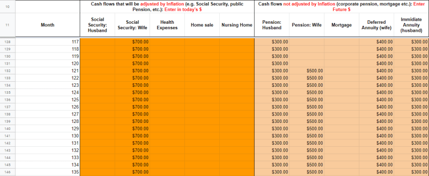
So, how do we enter all the future cash flows into the sheet? Very simple: this is the same setup as in the big SWR Google Sheet, see my SWR Series Part 28. Go to the tab “Cash Flow Assist” and enter all the relevant data. Notice that just in my other Google Sheet, there’s a distinction between “real, inflation-adjusted” cash flows and “nominal, not-CPI–adjusted” cash flows. I reserved space for 5 cash flow columns each. You don’t have to use all of them or you can add more of them by adding columns if you run out of space. Though, please make sure that you erase all the existing data in those columns if you’re using this sheet for your own calculations! 🙂
Real Cash Flows:
- Social Security Husband: Enter $2,500 between months 145 (filing) and 360 (assumed death).
- Social Security Wife: Enter $700 between months 85 and 360 and $2,500 afterward when the wife gets survivor benefits.
- Health Expenses: Starting in month 241, enter -$2,000, i.e., a negative number to account for the drag from additional health expenses later in retirement.
- Home Sale: A cash flow of +$300,000 in month 360
- Nursing Home: a negative cash flow of $2,000 every month starting on month 361.
Nominal Cash Flows:
- Pension Husband: Between month 85 and 360: Enter $300 for the husband’s pension. Notice that we assume that the wife will receive no more benefits
- Pension Wife: Starting in month 121, enter $500
- Mortgage: For the first 96 months, enter -$1,800
- Deferred Annuity for the wife: Starting in month TBA, enter
- Immediate annuity for the husband: Enter $300 between months 1 and 360.

Next, we head to the main tab and enter the main parameters. Only five of them:
- The expected inflation rate: 2.00%
- The (nominal) discount rate used in the NPV calculations: 4.00%. This is arguably the most important parameter, so bear with me on this one. We will check how different discount rates will impact your retirement budget.
- The horizon: 480 months
- The (financial) portfolio today: $1,500,000
- The bequest motive, i.e., how much money should be left over at the end of month 480. This is the money to be used as a cash reserve in case the last-surviving spouse lives beyond age 95 and/or money to leave to the kids.


And that’s all we need! The Google Sheet will compute the rest for you! No finance, no simulations, no asset allocation, no other fancy finance lingo!
So, let’s look at the results, see the screenshot below
- The top of this table is our household balance sheet with a column for assets and liabilities (ignore the column on the right for now).
- The Sheet automatically assigns the net present values from the 10 columns in the other tab into assets and liabilities. For example, the discounted value of the husband’s Social Security is about $361k (=asset). Or the discounted value of the future nursing home expenses represents a $232k liability.
- The row “equity” is calculated to “balance” the balance sheet, i.e., to make the sum of assets equal to the sum of liabilities. Hence, the “equity” portion is simply the sum of all the assets minus the sum of the non-equity liabilities. (and, yes, the equity is listed in the liabilities column. It’s not a mistake, it’s intentional. The way accountants always do this! And it makes sense in this context because the equity will be used to for outflows from the portfolio, i.e., your retirement budget, so it should be a liability!)
- If we subtract from our equity the discounted value of the bequest, just under $138k, we arrive at a pot of $1,750,891 that can be used for our retirement budget. (side note: one could also declare the bequest target as a liability on the balance sheet. Then the “equity” portion is what’s left for consumption. But I always consider the bequest a less explicit liability, more of a voluntary thing)
- How do we transform this fixed pot of money, into a retirement budget? Very simple, we calculate the present value of $1 of real consumption (i.e., $1 in the first month, then adjusted for 2% p.a. inflation going forward for another 479 months), which is $334.03 in this example. So, we simply have to divide $1,750,891 by 334.03 to get our monthly retirement budget of $5,242, or $62,900 per year.
- Quite intriguingly, the annual budget as a percentage of today’s portfolio is not too far away from the 4% Rule!


Technical note, for the spreadsheet wonks: All of the calculations boil down to using the Excel SUMPRODUCT formula, see the rows 5-8 in the “Cash Flow Assist” tab. For example, for the “real inflation-adjusted” series we calculate a SUMPRODUCT over 4 column vectors: 1) the series of cash flows, 2) the CPI index, 3) the discount factor and 4) an indicator variable that’s 1 if we’re within the retirement horizon and 0 beyond the retirement horizon. And for the nominal (current dollar) series we use only 3 column vectors, i.e., we skip the CPI-multiplier. It’s really that trivial!!!
Also, for every position in our balance sheet, we can calculate the impact it would have on the annual consumption target. That’s the column on the right (“Annual Cons.”), which is, in effect, the attribution of annual consumption coming from the different sources of wealth. For example:
- $53,887 comes from the financial portfolio,
- $12,979 from the husband’s Social Security,
- There’s an $8,335 drag due to the nursing home budget, etc.
- Even though the house is worth $300k today, you can factor in only about half of that in today’s net worth (about $152k). The rest is the opportunity cost of having the money tied up between now and finally selling it in retirement!
- All of these calculations are really simple: just divide the level entry in the balance sheet by the $334.03 factor to get the monthly attribution. Multiply by 12 to get the annual contribution.
Just a few words of caution: There are a few ways one could mess up this calculation. For example…
- Avoid double-counting! Notice that I included the mortgage as a negative cash flow on the balance sheet. Make sure you don’t subtract the mortgage a second time your current portfolio value!
- We will not count the primary residence in today’s $1,500,000 portfolio value. That’s because the home does not pay us any investment returns and it would be double-counting because we also count the (discounted) sale of the house as an asset.
I really like this approach because it’s so simple and intuitive. Especially the attribution is really informative. Lots of people always ask me questions like:
- What’s the value of my pension? Answer: see the NPV calculations!
- Should I count my primary residence in today’s Net Worth: Answer: No, because it’s not generating financial market returns. But completely ignoring would be too conservative. You can and should factor in a future home sale. In this particular example, about half of today’s home value can be factored into the balance sheet!
- I have a nominal (not CPI-adjusted) corporate pension. How much money should I set aside to “make this a real, CPI-adjusted pension”. Answer: look at the difference between a pension with and without COLA.
What’s not to like about this approach then? There are at least two problems with this approach.
Problem 1: The Discount Rate
How sensitive are my results with respect to the discount rate? Let’s look at a range of different discount rates and see how the annual retirement budget changes in response to the different rates.
- 2%: the current interest rate on intermediate government bonds (e.g. 10-years). Actually, it’s even a little bit below as we speak, but let’s round that up.
- 4%: my initial baseline. Clearly a higher yield than a pure safe government bond portfolio. Even higher than most investment-grade corporate bonds. So, to justify a 4% discount rate we’d need some higher-return assets in our portfolio, e.g., equities and/or real estate!
- 6%: If I were to assign an 8% expected nominal return to equities and 2% nominal to bonds, then a 2/3 stock & 1/3 bond portfolio would give you exactly a 6% expected return.
- 8%: With a more equity-heavy portfolio and maybe pushing up the equity return a little more, one could get to maybe, maybe 8%. Recall, the very long-term equity real return was about 6.7% p.a., so plus 2% inflation would get you to above 8%.
- I don’t advise going any higher than 8%. I know that some clueless people out there point to much higher historical averages (see my post from earlier this year How To “Lie” With Personal Finance for examples), but here on the ERN blog, we don’t fall for that!
So, what’s the range of retirement budgets for the 2-8% discount rates? Please see the chart below. Wow, that’s a huge range: $44k to $104k per year! If we were to go from a 4% discount rate to 3%, we’d reduce the retirement budget by over 15%! Go all the way down to 2% and we’re at about $44k. 30% less than the budget with the 4% discount rate, ouch!!!


But here’s the good news; I can also pump up our retirement budget if I set the discount rate high enough. This actuarial calculation reminds me of that old economist’s joke:
A mathematician, a quantum physicist and an economist are asked: What is 2+2? Here are their answers:
Mathematician: “4”
Physicist: “Somewhere between 3.99 and 4.01” (Heisenberg!!!)
Economist: (closes the door, closes the blinds, whispers into the ear of interviewer) “What do you want it to be?”
So, we can really make the retirement budget anything we want. Then, what should we pick as a suitable discount rate? So, here’s the bad news: even if you’re an accountant and/or actuary and you absolutely despise finance you can’t escape the realities of financial markets. You still need to set a discount rate based on financial market assumptions. Getting this parameter wrong will render the entire calculation worthless because small changes in the discount rate will have a tremendous impact on the sustainable retirement budget. We face a really serious GIGO (garbage in, garbage out) problem here!
So, what are the best practices in setting your discount rate? Just to be sure, actuaries do have some guidance:
“Setting the discount rate involves constructing yield curves from the raw trading data. As an overview, this involves calculating the yields-to-maturity using traded Government Securities. Different traded bonds will have different YTM, depending on the term of each bond and therefore yields would be different for each term. They would then need to be smoothed, interpolated and extrapolated to produce the full yield curve. The discount rate chosen from the derived yield curve will be based on the expected duration of the asset / liability.” Source: Numerica Consulting
So, actuaries recommend you first determine the duration of your cash flows. Notice this is not the 40-year retirement horizon, but the weighted average of the times when we realize the cash flows, so probably somewhere around smack-in-the-middle at around 20 years. Then simply look up the bond interest rate at that 20-year horizon. Using government bonds (U.S. Treasuries) will put us right around 2%. Whoah, with a 2% discount rate we can withdraw only a tiny $43,931 per year, which is only 2.93% of our $1,500,000 portfolio today! Even stingy old Big ERN never recommends a Safe Withdrawal Rate that low. Even with investment-grade corporate bonds, we’ll have a hard time getting to a 4% withdrawal rate. I looked up the average yield-to-maturity of the IGLB ETF (iShares Long-duration Corporate) and it’s about 3.60% right now. That would imply a retirement budget of $59k annually. Less than 4% of the current portfolio!
Side note: My blogging buddy Actuary on FIRE did a case study on a pension evaluation, actuary-style and back then (two years ago) he used a 4% discount rate when the overall interest rate level was about 0.5 percentage points higher. So, probably, 3.5-3.6% today is not too far off from what an actuary might use!
OK, so, that wasn’t really helpful. But again, we’re not bound by what actuaries recommend. It’s not like the American Academy of Actuaries will send their SWAT team to your house if you do your NPV calculations in violations of their best practices. So, we can certainly tie our discount rate closer to the expected portfolio returns. My suggestions for picking a discount rate: To account for Sequence of Return Risk we have to set our discount rate significantly lower than our average expected portfolio return, especially when dealing with highly volatile stock portfolios and esepcially after we’ve seen a bull market in its eleventh year!
So, in other words, if your entire portfolio consists of relatively safe investments, say, government bonds, TIPS, I Bonds, investment-grade corporate bonds, etc., then sure, use the quoted average portfolio yield as your discount rate. But as soon as you add equities, be very careful about going overboard with your discount rate. What may seem like a “safe” consumption budget today may not be so safe a year from now. This brings us the second problem with the NPV method…
Problem 2: Return Volatility and Sequence Risk
The second problem with the NPV approach is that the “safe withdrawal retirement budget” may not be so safe at all. There is no guarantee that if you recalculate the whole shebang again next year that you’ll end up with the same safe budget again. It might be higher, it might be lower.
Also, just for the record, the fact that a withdrawal strategy updates sustainable rates from time to time is not a deal-breaker at all. For example, I really like CAPE-based withdrawal strategies and, by definition, the rates computed that way will vary over time. So it’s not so much IF we have to change our retirement budget, but more a matter of HOW MUCH we have to change our budget over time and for HOW LONG we might have to tighten the belt if our portfolio underperforms.
So, let’s assume our sample retirement couple followed the advice of the actuary and starts withdrawing $5,242 per month from their $1.5m portfolio for a year. First, let’s ask ourselves under what circumstances would we NOT have to change our real CPI-adjusted retirement budget after 12 months? The answer is pretty simple: if the realized portfolio returns came in at exactly the discount rate, i.e., 0.3274% every month or 4.00% compounded annualized, then there’s no reason to change course.
I just did a quick calculation to confirm this: First, assume a 4% annual return for the first 12 months. This will get you a $1,476,775 in month 13, which I discount by 4% to bring it back into today’s dollars (about $1.42m). Then calculate all the remaining NPVs of cash flows the same as before but only for months 13-480. (technical note: this is all done from a month 1 NPV point of view. I could have also calculated this from the month 13 perspective with the same results)
Lo and behold, even though the net worth is now different, the consumption target is the same (in today’s dollars) as before because the PV of the $1 over months 13-480 is also slightly lower than over months 1-480.


So, the good news is that if your portfolio return exactly tracks your discount rate, then recomputing this actuarial SWR over time will always come back to the original safe withdrawal amount. Nice!
But that begs the question: What if my portfolio underperforms the 4% return target? That’s the next table! Assume that the return over the first 12 months was a cumulative -20%. Not even the worst bear market, but just a garden-variety bear market. Just look at the table on the right (and this is all the Google Sheet posted online!!!):


Well, not much of a shocker here: the portfolio is down substantially and your actuarial safe withdrawal amount after year one also has to be cut substantially. There isn’t quite a 1-for-1 relationship, though: the portfolio underperformed by 24 percentage points relative and the consumption target then drops by “only” 19.88% (inflation-adjusted). But it’s pretty darn close!
So, the “safe” withdrawal amount that your friendly accountant or actuary will calculate for you is safe but only as long as your portfolio doesn’t drop. Well, thanks for nothing! It’s like car insurance that’s only good as long as you don’t have an accident.
Of course, one can always argue that expected returns will rise after a large drop in the stock market. That’s because the next bull market will be right around the corner, hopefully! So, if we raise our discount rate in light of the drop to, say, 5% we still have to reduce the retirement budget by 10.8% relative to the baseline.


What is the “correct” new discount factor? Not sure! I’m also not sure if your actuary/accountant would know. In fact, if your actuary/accountant doesn’t understand equity valuations and exclusively looks at the bond yields as a reference for the discount rate, then he/she might make matters even worse; if the next recession and bear market work out the same as the past few then the Federal Reserve will likely lower (short-term) interest rates, go back to quantitative easing to drive down long-term interest rates, etc. which will lower the discount rate and that will lower the consumption budget even further and the drop in your real consumption will be even worse than the 19.88%. So much for a safe withdrawal amount!
Just as an aside, I really like CAPE-based withdrawal rule (see Part 18) as I mentioned here in the SWR Series before; you also lower your withdrawal amounts in response to a bear market, but you still raise the withdrawal rate, and you do so in a systematic and rational and intuitive way because expected returns are also higher at the bottom of a recession.
Back to the basics: The ERN SWR Google Sheet
So, what kind of safe withdrawal budget could this retired couple have sustained when looking at historical data? Very simple, I copy and paste the cash flow data into the SWR Google Sheet (see Part 28 for details). Also, assume that this couple has a portfolio with 70% Stocks and 30% Bonds (10-year U.S. Treasuries) and a 20% final net worth target ($300k=$1.5m*0.2). The historical fail-safe withdrawal amounts for the following at-risk cohorts would have been as follows:
- 1929: $67,543 (=4.50% of the initial $1.5m portfolio)
- 1960s: $67,627 (4.51%)
- 1972/73: $68,066 (4.54%)
Much higher than what a 2.0-3.5% discount rate in this actuarial exercise would have generated. In fact, we can reverse-engineer the discount rate for the NPV calculation that exactly matches the historical fail-safe withdrawal amount: With a 4.47% discount rate, we get to a $67,542 fail-safe retirement budget (close enough for government work).
But how would I have known that a 70/30 portfolio would require a 4.47% discount rate to be fail-safe in historical simulations? 4.47% is significantly lower than the average return of a 70/30 portfolio historically: 5.8% above inflation, so that would imply a roughly 7.8% nominal expected return. To account for Sequence Risk, we’d have to cut that down to 4.47%. So, again: one would never want to do a SWR analysis purely based on this actuarial calculation unless you actually have only low-risk assets (TIPS, I Bonds) in your portfolio and you’re prepared for a very, very lean retirement budget in light of today’s low bond yields. For most retirees, especially those in the FI/FIRE community with sizable stock allocations, simulations should be the centerpiece of retirement planning and these NPV calculations here would be a nice way of presenting the data afterward. Not more, not less.
Summary
I present this approach, not as an alternative to my simulation-based approach, but mostly as an add-on. I would never, ever use this NPV/actuarial approach on a stand-alone basis. It’s garbage in, garbage out: All of your results pretty much hinge on one single input: The discount rate!
Also, this approach gives me no guidance for my asset allocation. Quite the opposite, you might feel compelled to go for the highest risk asset allocation because it has the highest expected return and thus the highest discount rate which will likely generate the highest consumption target. But historical and Monte Carlo simulations show that you should keep a non-trivial share in safety assets, even if the expected return is somewhat lower. So, as much as you might dislike the simulation-based approach it still has to be an important component of our analysis. Maybe tag on this actuarial calculations afterward to gather some additional insights. For that, I’d definitely endorse this approach!