
Update 8/29/2018: Check out Part 28 as well with some enhancements to the Google Sheet!
Update: We posted the results from parts 1 through 8 as a Social Science Research Network (SSRN) working paper in pdf format:
Safe Withdrawal Rates: A Guide for Early Retirees (SSRN WP#2920322)
One commenter the other day had a good suggestion: Publish the Excel spreadsheet that we use in our safe withdrawal rate research. Great idea! There is only one problem: we didn’t use Excel to calculate any of the SWRs. We did use Excel to create some tables, but the computation and most charts were all done using GNU Octave, a free number-crunching programming language, similar to Matlab.
But we still liked the idea of creating a tool to run some quick SWR calculations. In Octave, we can calculate a large number of simulations and calculate safe withdrawal rates over a wide range of parameter value assumptions. Millions and millions of SWRs over many different combinations of parameter values (retirement horizons, final asset value target, equity shares, other withdrawal assumptions). That would have been cumbersome, probably even impossible to implement in Excel. But a quick snapshot on how one single set of SWR parameters would have performed over time? That’s actually quite easy to do, even though there are 1,700+ different retirement cohorts between 1871 and 2015.
Here’s the Google Sheet Link:
Link to the EarlyRetirementNow SWR Toolbox v1.0
For obvious reasons, the baseline Google Sheet can only be edited by us. If you like to run your own calculations you have to download your own copy. There are at least two ways to do so:
- (recommended) Click on Menu, then “Make a Copy” or “Add to MyDrive” to get a local copy of the spreadsheet in your own GoogleDrive. You can then edit the sheet and use your own assumptions.
- Click on Menu, then “Download as” then “Microsoft Excel (.xlsx)” to get a copy as an Excel file to store on your own hard drive. It’s not really recommended because most of the formatting will get lost. But if you care only about the computations you should be fine.
Update February/March 2017: Gold and cash returns
- Gold returns are only completely trustworthy after 1968 when I got the London Fixing time series via Quandl. Before that, I had to rely on annual data from OnlyGold.com. If someone has a better (monthly) time series for 1871-1967 please let me know!
- For cash returns I use:
- 3-month T-bill interest rates from the Federal Reserve starting in 1934. Monthly data.
- I have annual data going back to 1928 from NYU-Stern. Data gathered via Quandl.
- For 1871-1927 I use annual data on 1-year T-bill yields from Prof. Rober Shiller. It’s not exactly ideal to splice it this way but it’s the best I can right now. If someone has better data, please let me know!
How our tool is different from cFIREsim
- We use monthly data, while cFIREsim uses only annual data.
- We project forward return forecasts beyond 2016 year-end so we can calculate SWR for more starting dates. For example, the January 2000 cohort is already far underwater, as we showed a case study last week. Even aggressive return assumptions will still wipe out the portfolio before too long and we like to count those cohorts as 4% SWR failures even before the utter failure is actually confirmed.
- cFIREsim asks you for a specific withdrawal rate and then simulates how that rate would have performed over time for each of the different starting dates. We go the opposite route: We specify a final value target and our spreadsheet calculates the exact initial withdrawal rate that would have precisely matched the final value target. For every retirement cohort between February 1871 and December 2015 (=1,739 months). The advantage of this procedure is that we can then easily calculate the failure rates of different initial SWR without calculating any new simulations. The failure rate of the 4% rate? Simply calculate the share of ERN-SWRs that are greater than 4%. And redo the same for all rates between 3.00% and 5.00% without ever calculating any new set of simulations as would have been required in cFIREsim.
Enter Parameters
Fields with the orange shading are asking for user inputs:
- The Equity share. We are aggressive and set this to 90%. The residual is invested in 10-year U.S. Treasury Benchmark Bonds.
- The expense ratio: We currently set it to 0.05% p.a. One-twelfth of this is subtracted from each month’s return.
- Equity projected returns post 12/31/2016. These are real annualized return assumptions. In our SWR simulations we set this to 6.6% but here we are a bit more cautious and set this to a more conservative 5.0%.
- Bond returns: for the near-term (notice how low current 10Y yields are) and then longer-term. Short-term we use only 0.5% over the next ten years, then going a bit higher to 2.0% real return after that.
- Same for Cash: We expect pretty low cash returns over the next 10 years (0% real) and then a bit of a bump after that (+1% real).
- Expected future real return for Gold: We set this to +1%. Historically, gold has returned only about 1.5% p.a. after inflation.
- The length of the retirement horizon in months (e.g. 60 years = 720 months)
- The target final asset value as % of the initial portfolio. We set this to 50%.

Below the main parameters, you can also set an entire time series of additional cash flow needs (all monthly numbers as % of the initial portfolio value). For example, we predict to get a pension and Social Security worth about 1% of the initial net worth (in 2018 dollars) 25 years into retirement. So, starting in month 301 we set this value to 1%/12=0.0833%.

That’s all you need. The computer does the rest for you. It calculates the safe withdrawal rates for each month starting in February 1871 to December 2015 that would have exactly matched the final value targeting the last month of the retirement horizon.
Results
Some summary tables are in the first tab “Parameters & Main Results.” Be patient, depending on the internet connection and computer speed it may take a few seconds to recompute all results!
In the table on the left, we calculate the failsafe safe withdrawal rate both over the entire sample and for retirement cohorts post-1950 as well as the 1st, 5th, and 10th percentile. For example, since 1950, a 3.61% withdrawal rate would have failed 5% of the time and succeeded 95% of the time.
On the right, we calculate the failure probabilities of specific rates between 3% and 5% in 0.25% steps, again over the entire sample and since 1950, but also in the three CAPE regimes (<20, 20 to 30 and 30+). In the CAPE 20-30 regime, notice the big jump in the failure rates once you go beyond 3.5%!

We also throw in a chart with the data in the right table:

Distribution of the final portfolio value
In the tab “Distribution of Final Value” we can also specify a withdrawal rate and see the distribution of final asset values (real, CPI-adjusted, as multiples of initial). In the example below, we use the 4% rule. We are mostly worried about the left side of the distribution, so final values between the minimum and median. Note how for the median retirement cohort the investor would have grown the portfolio to 8 times (!) its initial real value. The maximum final value would have been a staggering 62-times the initial value. But at the same time, almost 10% of the retirement cohorts ran out of money!

More results
Also make sure you check out the tab “SWR time series,” which includes the SWR for all 1,700+ months in the simulation. For a quick look, there’s a time series chart as well. Notice how there are quite a few times when the SWR is quite substantially below 4%!

How the hell do we calculate so many SWRs?
Or, in other words, where’s the mega-spreadsheet that has 1,700 rows and 720 columns to iterate over the 60 years worth of portfolio values for the 1,700+ cohorts? We don’t need any of that! The withdrawal rate arithmetic is much easier than that. Stay tuned for next week’s post: our technical appendix with some of the background on the withdrawal rate arithmetic we developed. But if you’re interested, check out how the SWR tab “SWR time series” in Column E are calculated through some pretty trivial calculations from just four auxiliary variables in the tab “Stock/Bond Returns,” columns L through O. Likewise, we calculate the final asset values for the fixed withdrawal rate (column F in that same tab) without ever iterating over 720 months of returns each time we change the withdrawal rate. Much more elegant than the brute-force method in cFIREsim!
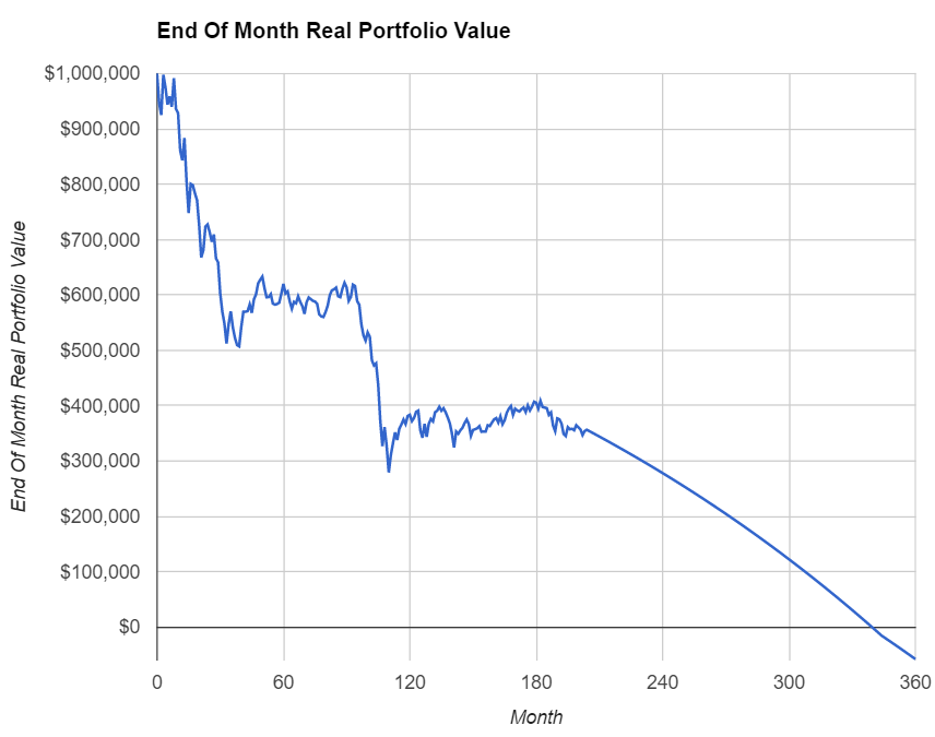
Case Study:
As we just mentioned, in calculating the SWR we never even go through the cFIREsim-style exercise of iterating over months and years and plotting the portfolio value time series. That would be too cumbersome for all 1,739 retirement cohorts and several decades of retirement horizon. But if you were wondering how any particular withdrawal rate would have performed over time for one specific retirement cohort, here’s the way to do it. Check out the tab “Case Study” where we can add the parameter values, again the orange shaded fields: The retirement start date (year/month), initial portfolio value and the withdrawal rate. And the computer does the rest!

The time series of portfolio values is in column D and also in the time series chart. This will use the same portfolio allocation and also the same supplemental income/expenses as in the main parameter tab. As we already noted last week, January 2000 would have been a pretty bad starting date for retirees. Not just early retirees!
Disclaimers
Please read the disclaimers here on the website and in the Google Sheet. We gladly grant the right for others to utilize our work but please make sure to credit us and quote us properly. We do own the copyright to everything we post here!
Also, note what this toolkit is and what it isn’t: It is a toolkit to determine how different withdrawal strategies would have performed in the past. It’s not a forecast. Past results are no guarantee of future results! But we can still learn from the past.
I’ve been exploring this spreadsheet – thanks for creating and sharing it! I’m particularly fascinated by the opposing nature of savers and retirees as it relates to Sequence of Returns Risk. What if I can be a saver during the first phase of early retirement through austere budgeting? It seems that we can explore this scenario by choosing a target portfolio value at >100% of the original. But there are a few aspects of your SWR Toolbox I’m not sure about that I hope you could clarify.
1) You describe the tab “Distribution of Final Value” as showing real dollars. In the main tab “Parameters & Main Results” is the ‘Final Value Target (% of Initial)’ in real or nominal dollars? I want to preserve 100% of my purchasing power after 60 years, not 100% of my nominal value.
2) As the portfolio grows faster through reinvestment of funds in excess of income & inflation, the safe yearly income will be higher than a portfolio that only grows to satisfy income & inflation. However many SWR studies choose the WR as a percentage of the original portfolio value, which is then adjusted for inflation over time but not adjusted for a growing portfolio. For a 100% asset preservation target, this seems fine — the portfolio only needs to grow to keep up with inflation. Does the math behind the SWR Toolbox allow for computing an additional growth factor separate from inflation that represents income growth through reinvestment? It seems that this would amount to a variable WR that grows relative to the original portfolio value over time, as opposed to WRs that vary with portfolio value at a fixed moment in time.
3) I’ve extended the spreadsheet with a coarse calculation for the yearly raise in income one would receive when the final target value is greater than 100%. This helps me explore just how low a WR I must commit to if I want a retirement income that increases faster than inflation. For a 2% yearly raise above inflation (growing to 328% of the original portfolio value after 60 years) it seems the SWR is quite low (1.6% for 0% failure). However this is a simple yearly compounding that doesn’t take into account sequence risk (or sequence benefit, in the case of a saver). It seems that another way to approach this is to provide numbers for Supplemental Income that represents the additional yearly savings due to austere budgeting. However this would be much more compelling if it were computed based on historical values like the rest of the SWR toolbox. For some retirement cohorts, the returns in early retirement are so poor that even low SWRs require spending capital instead of growing the portfolio; yet these are exactly the cases where being a saver (choosing an excessively conservative SWR) does best for the portfolio. Budgeting for an income that is a few basis points below the SWR during the first decade of early retirement should lead to a much better SWR later on. I’m curious what this dynamic looks like. Specifically I’m envisioning a scatterplot with one axis showing the basis point reduction (or increase) over the SWR for the first X years, and the other axis showing the basis point increase (or reduction) over the SWR for the remaining time. Ideally there won’t be a simple linear regression fit, due to compounding.
I’ve read your entire blog (not just the SWR series), so at this point I suppose I’m just pressing you for more material 🙂 Thanks for all that you’ve done, and I look forward to your future posts!
From this comment:
I’ve been exploring this spreadsheet – thanks for creating and sharing it! > I’m particularly fascinated by the opposing nature of savers and retirees > as it relates to Sequence of Returns Risk. What if I can be a saver during > the first phase of early retirement through austere budgeting? It seems > that we can explore this scenario by choosing a target portfolio value at > >100% of the original. But there are a few aspects of your SWR Toolbox I’m > not sure about that I hope you could clarify. > > 1) You describe the tab “Distribution of Final Value” as showing real > dollars. In the main tab “Parameters & Main Results” is the ‘Final Value > Target (% of Initial)’ in real or nominal dollars? I want to preserve 100% > of my purchasing power after 60 years, not 100% of my nominal value. > > 2) As the portfolio grows faster through reinvestment of funds in excess > of income & inflation, the safe yearly income will be higher than a > portfolio that only grows to satisfy income & inflation. However many SWR > studies choose the WR as a percentage of the original portfolio value, > which is then adjusted for inflation over time but not adjusted for a > growing portfolio. For a 100% asset preservation target, this seems fine — > the portfolio only needs to grow to keep up with inflation. Does the math > behind the SWR Toolbox allow for computing an additional growth factor > separate from inflation that represents income growth through reinvestment? > It seems that this would amount to a variable WR that grows relative to the > original portfolio value over time, as opposed to WRs that vary with > portfolio value at a fixed moment in time. > > 3) I’ve extended the spreadsheet with a coarse calculation for the yearly > raise in income one would receive when the final target value is greater > than 100%. This helps me explore just how low a WR I must commit to if I > want a retirement income that increases faster than inflation. For a 2% > yearly raise above inflation (growing to 328% of the original portfolio > value after 60 years) it seems the SWR is quite low (1.6% for 0% failure). > However this is a simple yearly compounding that doesn’t take into account > sequence risk (or sequence benefit, in the case of a saver). It seems that > another way to approach this is to provide numbers for Supplemental Income > that represents the additional yearly savings due to austere budgeting. > However this would be much more compelling if it were computed based on > historical values like the rest of the SWR toolbox. For some retirement > cohorts, the returns in early retirement are so poor that even low SWRs > require spending capital instead of growing the portfolio; yet these are > exactly the cases where being a saver (choosing an excessively conservative > SWR) does best for the portfolio. Budgeting for an income that is a few > basis points below the SWR during the first decade of early retirement > should lead to a much better SWR later on. I’m curious what this dynamic > looks like. Specifically I’m envisioning a scatterplot with one axis > showing the basis point reduction (or increase) over the SWR for the first > X years, and the other axis showing the basis point increase (or reduction) > over the SWR for the remaining time. Ideally there won’t be a simple linear > regression fit, due to compounding. > > I’ve read your entire blog (not just the SWR series), so at this point I > suppose I’m just pressing you for more material 🙂 Thanks for all that > you’ve done, and I look forward to your future posts! >
oops – please delete this weird self-reply
I performed some coarse calculations to examine the effects of a WR that is lower than the SWR, which leads to surpluses that are reinvested to grow the portfolio faster than inflation. Comparing this Austere Withdrawal Rate to the SWR over time shows that the yearly income generated by the AWR eventually surpasses the SWR, and this can take a long time (>10 years) for the tail case. However, here’s a big gap in the Final Portfolio Value between the tail case (safe 0 percentile) and even the 5% level. Since I’m exploring the possible upside from a low WR early on, I’m willing to take a look past the lowest “safe” upside amount. At the 5 percentile it takes a fraction of the time for the AWR income to surpass the SWR income. When comparing an SWR of 2.68% (for FV = 100% of original) to an AWR of 2.44% (nearly 0.25% difference), the tail case takes 14 years for AWR income to win, compared to less than 5 years for the 5 percentile.
My results are visualized here: https://public.tableau.com/profile/datanerd#!/vizhome/SWRvsAWR/YearsuntilAWRpayoff
Thanks! I provided the math for calculating the exact initial SWR with growing or declining the withdrawal amounts by rates over/under CPI. See SWR series part 8. Maybe you like to play with that!
Thanks!
1: all numbers are always in real, CPI-adjusted terms.
2,3: I have done some calculations for changing the withdrawals by less than inflation, see SWR part 5. This feature is not in the SWR Google Sheet, though.
But there is a relatively simple rule of thumb: If you increase the withdrawals by x% over and above inflation you’d have to decrease the SWR by about that same number.
For more on the math, see SWR series part 8 under “Time-varying withdrawal rates”!
Looking at part 5, I note that the WR changes to provide for different levels of consumption. I’m instead exploring a fixed WR at a level lower than the SWR, in order to fuel increasing consumption by way of portfolio growth through reinvestment. My WR could remain lower than the SWR perpetually, and eventually my smaller consumption of a larger portfolio would outpace the larger SWR consumed from a smaller portfolio. I’ve been digging in to determine if the payoff happens quickly enough to be worth considering, given the up-front lifestyle commitment it would require.
If you pick the WR and apply that same % every year, that would certainly do the trick provided you keep the WR below the target real portfolio return!
Hi, great posts so far. I’m new to this and trig to wrap my head round all the info. 1) So if I understood this correctly, in practice, when I’m coming up to retirement, I could input all the numbers into the parameters in the Google spreadsheet, look at what the CAPE will look like for the next 10 years and then check the spreadsheet in the 1st sheet entitled parameters and main results to see what could be my SWR? 2) I am looking to retire in approx 10 years, so I could use the tool from now to see what value my portfolio would need to grow to have my desired SWR? 3) I am an EU citizen so I’m wondering to what extent this can generalised to Europe? Im holding a world stock etf and global gov bond etf. I’m thinking using your spreadsheet and cfiresim which allows for more global portfolios. Cfiresim says with my pension contributions – 4% gave a 0% failure rate. With your spreadsheet I get 3.5% with max 5% failure rate. But that makes a big difference in terms of how long I work and I’m not sure what to go with. What do you suggest? Thanks a lot!
This spreadsheet is set up to work for simulations at the beginning of retirement. I would not recommend using this to plan your path to ER in 10 years. What you could do is set a “reasonable” portfolio return, iterate that forward 10 years and see where you stand in terms of portfolio value.
My sheet allows you to enter the pension income as % of the initial portfolio. The pension would then reduce your portfolio withdrawals in the future. Careful with nominal vs. inflation-adjusted pensions!
Hiya
1) So I could take the spreadsheet just before I retire, plug in the numbers and will know what SWR I should use by looking at what the CAPE would look like for the next 10 years? Eg cape 20-30 Quill tell me 5% failure rate if I withdraw 3.5%?
2) when inputting pension into the spreadsheet, let’s say I know that I would get eg USD1k/ month. So I would convert it to an annual amount and then divide it by my initial portfolio eg USD1M=0.012. I then input that and should divide it by 12?
1: correct
2: you input the monthly supplemental income (positive numbers) or expenses (negative numbers) as % of your net worth at retirement. So if you have $1m and expect $1,000 in monthly benefits then this would be 0.001. Or 0.1%.
Just out of curiosity Why is the supplemental income done as a percentage of original net worth as It is unlikely that whatever income you get has any relationship to net worth
In the new version (see SWR Series Part 28) I changed it to make this easier to input.
Aside from that: you have to input numbers. Whether you input them in $ or in % of today’s net worth, doesn’t really matter. It’s the same result.
Hiya
1) So I could take the spreadsheet just before I retire, plug in the numbers and will know what SWR I should use by looking at what the CAPE would look like for the next 10 years? Eg cape 20-30 Quill tell me 5% failure rate if I withdraw 3.5%?
2) when inputting pension into the spreadsheet, let’s say I know that I would get eg USD1k/ month. So I would convert it to an annual amount and then divide it by my initial portfolio eg USD1M=0.012. I then input that and should divide it by 12?
Thanks
A few questions regarding the Case Study calculations:
1) It appears that there aren’t any CAPE rules applied to the monthly withdrawel rates.The withdrawel amount remains constant based on the initial withdrawel rate. If I chose an intial withdrawel rate of 4% with a starting portfolio value of $1M, then I will see a monthly CPI adjusted withdrawel of $3,333 for the duration of the retirement horizon. Is this correct?
2) I entered a supplemental income and noticed the monthly withdrawel amount remained at $3,333 for all months regardless of the months which incurred supplemental income. Shouldn’t the monthly withdrawel amount be reduced by the supplemental income?
fantastic update, would like to know the details of the S&P drawdown and cashflow additions.
Perhaps you could post your Octave files on Github? Putting it in a Jupyter notebook would also make it more accessible.
Are you aware of any data sources that provide dividend and distribution history in addition to total return? This would be useful in incorporating tax drag into back tests.
Well, for the average FIRE person, running the whole Matlab/Octave gauntlet is probably overkill. That’s why I created the spreadsheet here.
Prof. Shiller has the SPX data (both price return and total return), so if you like you can gather the monthly dividend income from his spreadsheet.
I post the 10y benchmark returns in my spreadsheet. If you compare it with the 10y yield data on Prof Shiller’s you can also split that into yield vs. price return vs. total return
http://www.econ.yale.edu/~shiller/data.htm
A question about using the Toolbox v2.0: Somehow my results indicate that the CAPE>20 (I assume it should be 20-30) is riskier than CAPE>30. For example, at 5.5% WR, the probability of failure for CAPE>20 is 42.65%, but was 0% for CAPE>30. At WR 5.75%, the probability of failure is 53.01% for CAPE>20, and 32.2% for CAPE>30.
I played with the parameters I entered, and I found that these kind of results are mostly due to the fact that I had entered 45% as stocks. I wonder if the results are legitimate, or it’s due to a bug?
I am reading your PDF section 3.2-Simulation Results, and I noticed similar phenomenon for 30 yr horizon (but not for the 60 yrs). I set my horizon at 40 yrs, so I got similar results to your 30 yr simulation. So this is not a bug. 🙂
But why this happens? Why with a 30-40 yr horizon, and when CAPE is sky high, a bond dominant portfolio will have 100% chance of success?
Very interesting! I do a lot of data analysis on biological/medical data, and I see a huge similarity between the finance simulation and bio-data analysis.
Use the conditional failure rates with a degree of caution. There were only a few instances where the CAPE was this high and we observed failures.
It’s possible that for very high bond shares (and low=45% equity shares) the 1960s/1970s were the worst possible staring point, even though the CAPE at 25 was lower than in 1929 (CAPE >30).
It’s not a bug. That’s just how the stock/bond returns worked out. There isn’t a perfect correlation between CAPE and future returns! 🙂
An older response but I’m noticing the same thing as Shawn and am confused about your answer and concerned about my results.
I have some future (social security) cash flows entered but otherwise am just modifying the stocks vs 10y bonds parameters with a 480 month horizon.
As I change the asset allocation, the SCR for the 0% failure rate for CAPE>20 & SPX ATH has a maximum. For example, below are what I saw for SCR for these different stock and bond allocations (first digit is % stock, second is % bond).
You can see it maximizes at around 60/40 stock/bond allocation.
My main question is whether this type of analysis makes sense or if this is incorrect usage.
Something just doesn’t feel right about this. For one thing it points to an optimal asset allocation which I don’t think exists. For another the SCR (while I know is generally pretty sensitive) seems overly sensitive to the asset allocation. And lastly it seems like this conflicts with your glidepath analyses.
0,100: 3%
10,90: 3.25%
20,80: 3.25%
30,70: 3.5%
40,60: 3.75%
50,50: 3.75%
60,40: 4%
70,30: 4%
80,20: 3.75%
90,10: 3.5%
100,0: 3%
Yes, that’s how I would look for the optimal asset allocation. I would probably check 65/35 to see if this yields an even larger SWR.
I don’t share your concerns you stated in your last paragraph:
If you specify an objective function then an optimal asset allocation exists. For maximizing the SCR, you normally get an optimal interior solution around 60-75%.
Yeah, the SCR is sensitive to the asset allocation. As it should be.
No it doesn’t. If you check in part 19, the large table has the optimal asset allocation at 75% for static weights. But a GP beats that slightly. You didn’t even show me any GP SCRs, so how do you know how a GP would perform?
Found this sheet, which led me to the rest of your site (loving it!). The sheet is extremely helpful as I am 9 months away from FIRE (been FI for a while, but finally getting around to retiring early). I am having a file problem and I am hoping it is no big deal. When I copy, no issues. But when I saved the file and opened it, I get an error.
“Excel completed file level validation and repair. Some parts of this workbook may have been repaired or discarded.
Removed Records: Formula from /xl/worksheets/sheet1.xml part”
This is what popped up. It had a link to a file, so this is what is in it.
error322800_01.xml
Errors were detected in file ‘E:\Users\Scott\Downloads\Copy of EarlyRetirementNow SWR Toolbox v2.0 – save your own copy before editing!.xlsx’
–
Excel completed file level validation and repair. Some parts of this workbook may have been repaired or discarded.
–
Removed Records: Formula from /xl/worksheets/sheet1.xml part
Using Office Pro Plus 2016 and I know that isn’t the very latest (if you count 365), but it seems too recent for that to be the issue.
Thanks again, terrific product that on initial look might mean I withdraw a higher number than I was thinking (I was thinking 3% since I will be 54, but might go just below the worst failsafe).
Oh wow, I can not guarantee any conversions, especially not to older versions of Excel. No idea why that happens. I occasionally export this to Excel and the formulas work. But the formating is completely messed up. So I just keep all the calculations in Google Sheets…
Big ERN, love the site and the SWR series. We RE last November and were living the 4% rule until I stumbled here.
I am 52, married with 62k pension. NW is $1.1m.
Looking to take SS @ 62, approx 22k. Mrs @ 62 for 16k.
Is it possible I am looking at 11% SWR at 60/40 or did I screw something up with your calculator?
Keep up the great work bringing clarity to the masses.
Doesn’t look too crazy. It’s because you almost fund that $121k annual budget with your SS alone 10 years down the road.
But make sure you account for the pension as a nominal (non-COLA) cash flow if it doesn’t have COLA.
Also, make sure you check if it isn’t optimal to use different timing on the SS. Normally, the higher earner to take benefits at age 70.
Check https://opensocialsecurity.com/
Love the site and SWR series. I do have a question about the term SWR in the spreadsheet.
Using defaults with a 0% target and a $2M NW, the spreadsheet calculates “0% Failure Rate – All” as about 3.19% and $5311/ month. If I add $1000/month of COLA income to the scenario, the SWR goes to about 3.79%.
It seems to me that the 3.79% figure is more of a safe spending rate than a withdrawal rate. It really means that I will withdraw safely at 3.19% and will supplement with $1000 to have $6311/month. The $6311 equates to 3.79%.
In fact, without the additional income, the SWR stays the same as I vary the NW.
Am I misinterpreting?
Correct. It’s the spending rate. 🙂
Big ERN, had a question wrt the assumption for the stock returns. Is that using the S&P or VTI? I noticed you have small and value listed as well.
How would you model for a portfolio consisting of the stock allocation split between US Total index, Small cap value, Emerging, Developed and US REITS (Eg: VNQ)?
S&P 500. It’s the index where I had a long enough return history.
If you want to model different indexes (REITs, Total Market, etc.), you’d likely have to do a regression analysis and estimate the appropriate factor exposures to the base factors I use.
For example, REITs will likely look like a leveraged equity+bond portfolio. VTI will look like S&P500 plus a minor long exposure in small-cap stocks, etc.
I haven’t written about those issues yet but it’s on my to-do list. 🙂
Correct me if I am wrong but I believe as long as the total allocations to REITS, small cap value are less than 20% of my total stock portfolio; it should not have a material impact on a 60 year retirement with 3% SWR?
I am worried about the Developed (ex-US) and Emerging allocation in my portfolio. I looked at random periods and did not get a consistent feel for their returns. Also given the severe under performance in the recent decade coupled with the China heavy exposure in Emerging and Commodity/Utilities exposure in Developed has me second guessing myself for the future. Dump them now or live with reduced drag going forward is my worry. Also if there is a threshold not to exceed for Ex-US funds?
Will wait for your future posts and hopefully I do not need to end my early retirement and go back to work based on your data 🙂
EM and non-US developed do not consistently underperform the US. They have done so over the last few years, but for example, post-2002 they did very well.
It’s a tough call: hang on to the losers and hope this reverses again (as has happened many times before) or risk even more years and decades of underperformence?
I’d suspect that anything China-related will be toxic for a while. But some other EM countries: India, Vietnam, Philippines, Indonesia, etc. will pick up the slack.
I am a long time reader but first time comment. I am almost a number geek myself (but not to the extend of Big ERN) so thoroughly enjoy the SWR series.
I recently came across an old article (2013) where the author suggested that 10 years equity return is predicted by “average investor equity allocation %” rather than the very commonly used metrics such as S&P500 P/E or CAPE.
http://www.philosophicaleconomics.com/2013/12/the-single-greatest-predictor-of-future-stock-market-returns/
FRED has this chart that refreshed till Apr this year (2020).
https://fred.stlouisfed.org/graph/?g=qis
I find the study fascinating, and since the first 10 years return is the key to a successful withdrawal due to Sequence of Return Risk, I took the SWR series from Big ERN and plotted against the inverse of investor equity %, and found that it tracks the SWR very closely. The only big exception is during 1950 to 1970, maybe due to the much higher inflation rate back then? Though it certainly fit SWR much better than CAEY.
https://docs.google.com/spreadsheets/d/1hirqlrcC_QIW7ANUj76r7JgBDmGH0Z9LMpMQdlrtzdk/edit?usp=sharing
If it is indicative or next 10 years return, the April number would have predicted almost exactly 4% withdrawal rate. But given that market has already risen by 50% since April, it is also unclear what would be the latest prediction until it is updated.
Not sure if Big ERN has seen this study, and can you take a stab if this allocation % is making any sense?
Thanks for the link. I had seen the study before. Very interesting.
The two indicators 1) CAPE and 2) equity allocation are both predictive of future returns. The fact that 2 predicts the market doesn’t mean that 1 is useless. They are both useful. They are both useful because they are obviously correlated not just statistically, but also fundamentally because a high CAPE is due to the long equity bull market which also drives up the equity allocation.
The problem with your proposed indicator: It has a 2-quarter lag. I prefer an indicator that can be constructed in real-time over the one with the higher correlation but with a 2q-lag.
But I agree: this chart is quite intriguing. I will certainly look at this some more and maybe write a blog post about this. Thanks for the reminder! 🙂
Can’t wait to read your assessment 🙂
Have you considered making asset allocation an output instead of an input?
Asset allocation appears to have a large impact on SWR / Failure rate but I think myself and other readers care much more about SWR and Failure rate than Asset Allocation. I care about asset allocation only to the extend that it affects those two things! Personally I think it makes the most sense to enter Failure Rate as a single input and then output % equities in a table as a function of SWR Rate and CAPE ratio. Have you considered that or is there a reason why that wouldn’t work?
Thanks!
With the current setup that’s likely not feasible. But entering a few asset allocation choices in 5% steps you will get to the “optimal” allocation quickly.
But: I warn that tailoring the AA too much might result in overfitting. That’s the mistake people like Bengen make, where they say Small and Value stocks would have done better. That’s overfitting and junk science.
I’ve wondered this same thing myself about asset allocation (where equities share is a function of equity valuation).
Using a hacked copy of the Case study tab, I’ve been modeling having equity share vary between 60% and 100% based on a relatively simple function of how much equities are off their all-time high, i seem to see nice incremental improvements in SWR for all years since 1946. (It does *not* work for the Great Depression / before Fed monetary policy was changed to prevent sustained deflation).
I suspect it’d be better still rebalancing only every 3 to 6 months, to capture momentum, per Part 39, but I’m not sufficiently proficient at Excel to figure out how to model that.
Can I have you check my math? We will retire at me age 53, wife 45 (same year as we are 8 years apart.) My pension at age 62 will be (in real dollars) 18000, social security at my age 70, her age 72 will be a total of $3300/mo. If our starting net worth is 2.5 million, then at month 108 (9 years after retirement), will draw the $18000 pension which would be 0.06% of initial net worth/month and then at my age 70/wife 62 we will then add $36000 of social security income and thus at month 204, i should have 0.18% net worth/month. If thats right, my SWR just became alot better!! Thanks for all of this free info in the form of your brilliant series of posts!
Sorry that should say “my age 70/her age 62)
Gotcha!
That sounds about right. Glad that the SWR got better. But it shouldn’t rise by more than 0.10%, certainly not more than 0.18%
Only 0.12 but its something!
Just to say, thanks Big ERN for putting this together, what an amazing piece of work. The inclusion of non-US stocks is also greatly appreciated, for those of us who are VWRL-ing our way into retirement…
And after an afternoon with your spreadsheet I have a lot more confidence in our SWR and pulling the pin on early retirement…
Thanks, Mike! Glad this is useful!
Good luck with your FIRE planning! 🙂
thank you so such a comprehensive tool and the explanations. How should one handle one time cash increases such as inheritance. I added the amount in a future year in column J/’cash flow not adjusted for inflation’. This creates a negative withdrawal amount for year of the inheritance and lowers the necessary withdraw amount every year afterwards. The model uses the positive cash flow to offset withdraw amount and rate, but does not appear to be adding the inheritance to net assets and therefor benefit from higher absolute market returns. Is this correct? Do you think it is significant? Is there another way to capture the benefits of future inheritance on the portfolio and total market return and not only on cash withdraw offset?
The model assumes that the assets will be added to the portfolio, in line with the portfolio asset allocation.
In other words, if you ask: “but does not appear to be adding the inheritance to net assets and therefor benefit from higher absolute market returns. Is this correct?” I’d answer, no that’s not correct. No idea where this allegation comes from. You most definitely add the amount to the portfolio.
Thank you for your excellent SWR spreadsheet. I’ve been using it for some time. I especially enjoy your recent appearances on Two Side of FI. I’ve been playing around with the latest version and I noticed one issue that you may have overlooked. If you have significant future cashflows, your failsafe SWR may be higher than 5% and this is fine, except that in the graph “Failure Rates of different Consumption/Withdrawal Rates” the pre-determined range is 3-4.75% so the graph is blank since there are no failures at these levels.
It’s a bug due the stupidity and incompetence of Google Sheets.
The WRs in the table in cells D8:D16 certainly adjust automatically based on the interesting range of SWRs. Essentially the overall failsafe, rounded down to the closest 0.25%. And then up 200bps in 25bps steps.
When you do a chart over that you have two choices: either let Google decide the x-axis range. Or specify the x-axis by hand. If you specify it by hand as done in my sheet, you need to go into the chart options and change it to your preferred range if you change the inputs.
If you let Google choose it then it’s way too wide, usually 0-10% or some other useless range.
Pick your poison. But it’s not my fault. Google and Excel should allow variable chart axis ranges. But they currently don’t.
Karsten,
I believe for the 10Y BM month over month returns that you use S&P-TR historical data. If I calculate a monthly nominal return from TR monthly closing data for 1985, I get -3.36, 2.52, and 2.39% for January through March. If I convert the Toolbox real returns, the nominal returns are -3.32, 2.52, and 2.39% but they are reported for February through April. This one month shift continues through the database. While I would expect the one-month shift in monthly returns has zero impact on your SWR results, from a purely academic standpoint why is there a shift in month over month returns?
Thanks for pointing this out. I have 10y BM bond data from 1790-2013 from another database. Then the S&P data from 2011. For the overlapping window 2011-2013 the two are very close together, so I was confident that the historical DB can be used to backfill all the way to 1871.
Do you have a database for S&P TR 10y BM you can share? Is this just one 3-month window that’s inconsistent? Is the entire sample pre-2011 shifted by 1 month?
Thanks in advance for any help!
I looked at the data in more detail. It should be pretty obvious in what month the large negative return occurs: When did we see a large increase the 10y yield?
According to the FRED database (https://fred.stlouisfed.org/series/DGS10) the 10y yields at month-end were:
Date Yield Diff
12/31/84 11.55%
01/31/85 11.17% -0.38%
02/28/85 11.91% 0.74%
03/31/85 11.65% -0.26%
04/30/85 11.41% -0.24%
Thus, the big jump in the yield occurred in February. That’s where I got the large decline in the index (-3.32%). Your January number has to be wrong. You can’t get a 3.36% drop in the index when the yield decreased by 38bps.
It looks like my numbers are correct. Yours are off by 1 month.
My calculations using the Yahoo 10Yr yields
https://docs.google.com/spreadsheets/d/1PN1LK-v9qyp_AVavQzueWYzjIWXEn6tDVvxr_L2qBrs/edit?usp=sharing
I must be making some wrong assumption as to returns for the start or end of the month. I follow your FRED explanation and just cannot reconcile with calculations using Yahoo data with bond return formula. Thank you for such a quick reply to my original post and for looking at the linked database.
Your yields have a time stamp on the 1st of the month. Everything I do is time-stamped at the end of the month.
Mystery solved. I will keep my numbers as is.
Thanks for checking! 🙂
Also, a lesson learned: Don’t use Yahoo Finance monthly data. Always use their daily data, then get the monthly numbers through the “vlookup” function at month-end.
Before posting my inquiry, I had verified the Yahoo 10 Yr BM monthly with daily data noting as you did that the timestamp for monthly data is the first day of the month. Even though the timestamp for monthly data defaults to the first of the month, the data at the close is correct for the last day of any month in question. In the same Google link I previously posted, I have a comparison of partial Yahoo daily (start and end of month) compared with Yahoo monthly data (with default first of month tie stamp). I still maintain there is a one shift between your database and returns calculated from Yahoo data for some reason that I cannot understand. I appreciate any feedback. Thank you Karsten.
Your calculations are incorrect. In the sheet, formula E8, why does the return in Feb 1985 depend on the yield at the end of March 1985?
E8 = (C8/C9+C8/1200+(1+C9/1200)^-119*(1-C8/C9))-1
And again: the large decline in the index has to occur in the month with the large yield increase/ Feb->Mar 1985 was the big jump in the yield, so my calculations are correct in putting the large decline in the index in Feb 1985. The fact that your TR index increases in Feb 1985, when the yield goes from 11.17 (end of Jan) to 11.91 (Feb 1985) should tell you that the return CANNOT be +2.52%. You are off by 1 month.
Hello Karsten: Thank you for creating this invaluable tool and for working with Jason to create a great tutorial. Could you help me with an issue? The toolbox lists 8 types of portfolio assets but I have a much more diversified portfolio than the items listed. One account includes US Mid, Small, Micro Stocks, US Value Stocks, Total US Stock Market, VTSAX, Developed International Stock, Long Term US Treasury Bonds, Emerging International Stocks, Cash, International Bonds, Aggregate US Bonds. Any suggestions for how to handle or represent within the asset types? Thanks so much.
Approximate factor loadings of asset classes not listed in the SWR sheet:
US Mid, Small, Micro Stocks, = 100% S&P plus 100% SMB
US Value Stocks = 100% S&P plus 14% SMB +100%HML
Total US Stock Market, VTSAX = 100% S&P plus 14% SMB
Developed International Stock = 100% International
Long Term US Treasury Bonds = 100% 30Y bonds
Emerging International Stocks = -1.8% S&P 500 -5.8% 10y Bonds +10.0% 30y bonds + 89.5% international + 18.0% Gold +13.5% SMB + 8.0% HML -9.9% Cash
Cash = 100% Cash
International Bonds. Not sure. Probably use US Agg Bonds
Aggregate US Bonds = 8.9% S&P500 + 58.0% 10y Treausry + 33.1% short-term cash
I have been using this sheet for a while, but I have noticed a contradiction. I have a situation where I expect relatively high income, starting when I hit 65, but when I put the data in the sheet, I see an enormous disparity between the SWR on the cash-flow-assist sheet and the cape-based-rule sheet. I simplified this as a test and I still see an enormous difference using all of your defaults ($10,589 vs $15,105). I understand that one can make changes each month in the latter and not the former, but the 50% difference seems too high; you’d be going through 1.5 times the money. And the starting CAPE ratio of 25 is historically high so you’d think this would be lower.
To recreate this, start from a clean copy of your worksheet. Then assume $10,000 in today’s dollars in income starting in row 254 (when the older spouse turns 70), and continuing perpetually. T11 on the cash-flow-assist sheet is 10,589, while b16 on the Cape-based-Rule is $15,105.
Would this be the expected result in that situation?
It’s not a contradiction.
I might have slightly different parameters, but here’s what I got. These are the safe withdrawal amounts as a function of the supplemental flows. I also calculate the marginal impact of each additional dollar of future flows. Notice how the marginal impact is constant, so the future flows have a linear impact on today’s budget. Only the slopes are different for Standard vs. CAPE:
SupplementalFlow 0 1000 2000 5000 10000
Standard $8,584 $8,785 $8,985 $9,587 $10,589
Marginal N/A 20.05% 20.05% 20.05% 20.05%
CAPE-based $10,323 $10,733 $11,143 $12,372 $14,420
Marginal N/A 40.97% 40.97% 40.97% 40.97%
You will notice that in the standard method (fail-safe), you have a very small impact from future flows. Only about $0.20 per dollar of future flows. That’s expected. The CAPE-based rule with a relatively low discount rate applies much more weight to future cash flows. That’s as expected.
Also notice that the SCR in the standard model is only marginally above your safe cash flows later in retirement. Thus, you almost wipe out the entire nest egg in the worst-case scenario. (SCR=10589 vs. 10000, so there’s only a tiny portfolio left to pay 589 a month once your benefits start).
Also notice that in this worst-case scenario, your CAPE-based withdrawals would have certainly dropped from $14 to less than 7k a month (see the worst drawdown = 53.22 in the table in the CAPE-based sheet).
It’s a tradeoff: CAPE-based allows you to withdraw more initially. But in the worst case, you experience drastic withdrawal cuts.
PS: mystery solved. I changed one number back to the default and I got your $15,105, not the initial $14,420. So, even a slightly higher slope for the CAPE rule. But the answer is still the same: CAPE has a lower discount rate. Thus the higher weight on future flows. But also very, very bad downside risk for your monthely withdrawals, 50% or more with the 1.75/0.50 CAPE parameters.
Thank you so much for the considered reply. I love how active you are in this forum!
I have one (well at least one) thing that I’m still confused about. In the chart at the top right of the CAPE-based rule sheet, it lists worst 30y change, drawdown, mean vs. initial, and volatility. What I really want to know, though, is what was lowest monthly withdrawal amount, compared to today’s withdrawal. (As I understand it, at the month of the lowest drawdown, the CAPE rate would be the lowest, which would mean that the actual amount withdrawn would be considerably more than the lower percentage). I guess the 30 yr worst mean vs initial is kind of what I’m looking for.
Does this make sense?
I don’t quite understand what you want. The stats in the table are the withdrawal amounts relative to the initial. So, if the worst 30y change is -53% is means that the lowest withdrawal amount was 53% below the initial withdrawal amount.
Sincere ‘Thank you’ for the years of work you’ve put into the blog, toolkit, and for sharing on various podcasts. I’ve been pouring into the SWR Series in the last couple weeks, as I’m possibly retiring in March.
Two questions about using the toolkit. I’ve re-read parts 7, 8, 28, and watched the Two Sides of FI video.
Scenario: I retire in five months, and my spouse continues working for four years.
1. How does one model one spouse working longer when the other spouse retires?
2. How does one capture actual spend (after the first person retires)?
From what I’ve read, I believe we would enter the following in the toolkit:
1. Set the Start Date to 3/1/2024
2. Enter $5,000 (example Spouse income) in Cash Flow 2 for the first 48 months (4 years)
3. Set Scaling Factor to 0 for those months [I’m not positive how Scaling Factor works. Plus, in bright red the column says not to touch it. 😊]
4. Before I retire, record any expected spending in either Cash Flow 1 or Cash Flow 3 columns
5. After I retire, record actuals in the same column chosen for #4.
Is this correct? My goals are to 1) model now, and 2) use the toolkit for the first several years of retirement to record actuals and adjust accordingly.
Thank you in advance,
Steve
Steps 1-3 are correect.
The sheet will give you an estimate of how much you withdraw starting at the time when the scaling is back to 1, presumably 3/1/2028.
There is no need to monitor realized spending in the Google Sheet. You should clearly monitor your spending to get e grip on your retirement budget. But as time passes, you’d move your “as of date” and roll the number of months with scaling = 0 down to zero. Past spending is lways just water under the bridge for the Google Sheet.
But yes, track your spending, just not in the Google Sheet.
I’m getting a minus value in my SWR column “T” for the first 28 months of my 431 month retirement. Most of my retirement income is from a pension and SS entered in columns “E” and “J”. My portfolio is only $170K. Not sure what this means.
That’s legit. If you enter your (positive) cash flows from SS and pension, it’s likely that the pension, due to a lack of COLA will be inflated away. So, your benefits are frontloaded and you want to consume less than what comes in and rather contribute to your portfolio. Then at month 29 you will draw on the portfolio (170k plus the small contributions form months 1-28) to make up for the inflation erosion in your corporate pension.
Using your sheet version 11/12/2203 (last two dates wrong in the Change Log sheet?).
Data entry question on “Cash Flow Assist” sheet: My wife’s SocSec will end when I die which is a different date than she dies. When entering SocSec (cells E & F). Do I copy amount from the starting cell to the end of the table or stop it when I expect each of us to die?
What affect does the “Retirement Horizon (Months)” value have on the “Cash Flow Assist” sheet?
Question about Expense Ration (p.a.) on sheet “Parameters & Main Results”. Is this really 0.05% (0.0005) or is this 5% (0.05)?
Is my assumption correct that this is the ratio of annual expense to portfolio? For example, a $40,000 per year expense with a portfolio of $1,000,000 would be 40,000/1,000,000 = 0.04 or 4%.
When considering expenses, should this include all income taxes including the taxes that may be generated when doing roth conversions?
Thank you so my much for the work you have done. I really enjoyed the sparring you and Fritz had reagarding the bucket strategy. I learned a lot from that blog. SAA is much simpler than buckets.
“Question about Expense Ration (p.a.) on sheet “Parameters & Main Results”. Is this really 0.05% (0.0005) or is this 5% (0.05)?
Is my assumption correct that this is the ratio of annual expense to portfolio? For example, a $40,000 per year expense with a portfolio of $1,000,000 would be 40,000/1,000,000 = 0.04 or 4%.”
I think I really missed the meaning of Expense Ratio. I think this is the average expense ratio for the funds, correct?
Correct!
1: changed the log date to 11/12/2023. Good catch!
2: You include the benefits of the first spouse to die only up to the expected death time. Then set it to zero afterward.
3: You can cut off the last survivor benefits at the appropriate date. Though, the sheet will cut off any cash flow from the cash flow tab after the retirement horizon you enter in the main parameter sheet.
4: The expense ratio is exactly that. In the default setting it’s 0.05%=0.0005. It’s certainly not 5%.
5: Taxes: this sheet is done pre-tax. If you expect to pay a mostly flat tax you may subtract that from the gross withdrawals to get your net retirement budget. If you expect large one-time tax burdens, like from Roth conversions in specific years, you should probably model those as negative cash flows in the appropriate tab.
So if i just use the fail-safe (do not consider CAPE), i just take that withdrawal rate, find SCR for my first year of retirement and can just change that withdrawal amount by inflation every year (assuming no cash flows that would reduce withdrawal amount)?
That is the idea, yes. You may also ratchet up the withdrawal amounts over time when you realize that the historical worst-case scenario didn’t repeat itself.
Appreciate you, sir
Totally dumb question again…if I do end up using CAPE adjustments instead of worst-case scenario SCR, do I multiply the suggested CAPE-adjusted withdrawal rate by my initial portfolio value or current? Do i just use that SCR or do I also add in an inflation adjustment or is that already considered when using the CAPE-adjusted rate?
The CAPE-based rule uses the current portfolio, not the initial.
In the CAPE-based rule there are no CPI adjustments. It’s the current portfolio times the CAPE-rule WR.
In your SWR calculations do you withdraw at the beginning or end of the month?
Beginning of the month, i.e., last trading day of the prior month you already take out the money.
Hi Karsten, This is an amazing tool, and I plan to use it as I’m looking to retire early (at age 58) in a few years. If you ever decide you’re “done” with all of this, how would one go about continuing the updates you make to prevent it from going out of date? 🙂
Apologies if that’s a dumb question or if it was asked and I missed it in previous comments. Thanks for sharing your knowledge and this incredible tool.
Good question. I’m not planning to quit anytime soon. If I ever change my mind I would not just do a rug-pull, but ensure a proper transition to new owner(s) who can take care of my “baby.” 🙂
Hi Karsten! I have a quick question on the sheet that I’m hoping you can clarify.
I am 59 and looking to retire at 60. I notice the sheet has 720 months. Do I need to fill in supplemental cashflows all the way to month 720 (I’d be 120!) or just to the “retirement horizon” I set in order to get an accurate SWR?
Thanks for all your great work!
Only up to your retirement horizon. Everything beyond that will be ignored in the calculations.
Thanks!
Really appreciate the SWR toolbox- it’s by far the best retirement planner I’ve found. One thing I’ve noticed is that your spreadsheet gives me more optimistic results than cfiresim. For example with a 75/25 portoflio, 45 year long horizon, .10% exp ratio and a 25% FV, the SWR toolbox calculates a failsafe WR of 3.29% (which occurs in 1929). If I enter that same scenario into cfiresim, it fails in one of the cycles (1966). If I use the “case study” tab in the SWR toolkit and set the start date to January 1966, I can see that the ending value is still $482k. Here’s a link to the cfiresim scenario: https://www.cfiresim.com/f4e3b5e2-2b3b-48d9-bd94-acb29b1472b7
Any idea why there would be such a large discrepancy? Is it just due to the fact that cfiresim only simulates annual withdrawals vs monthly? If anything, I would think that would make it more optimistic (since I believe it deducts the withdrawals at the end of each year)? As far as i know, you use the same Shiller dataset.
On a related note, I know you wrote an article about how the frequency of rebalancing affects SWR (iirc, there was a slight advantage overall to going with an annual vs monthly rebalancing strategy), but do you have inisght/data on how withdrawal frequency affects the SWR? I’m asking because I’ll likely do quarterly withdrawals (for convenience) during retirement but just want to understand roughly how big a difference this could make vs monthly.
Your numerical example shows that my toolkit is more conservative than cfiresim. 3.29% exhausts the nest egg in my toolkit, but leaves +$482k in cfiresim.
The reason is that cfiresim can’t properly simulate 1929 because it’s simulated annually, while mine is monthly. So cfiresim (and Trinity Study, and many others) can’t properly simulate the 9/1929 market peak.
I studied withdrawal frequencies in Part 47 and that makes very little difference: https://earlyretirementnow.com/2021/08/18/when-to-worry-when-to-wing-it-swr-series-part-47/
Ah- thanks for that link!
BTW- the scenario i was trying to describe when comparing the SWR tooklit to cfiresim is the opposite- in cfiresim my scenario fails in 1 of the backtests (1966). But in the SWR toolkit, I’m left with a minimum of 482k even in the worst case (9/1929). That’s what I’m trying to figure out…because if anything cfiresim should give more optimistic results due to only having annual data. Any other causes you can think of? Obviously, your part 47 article debunks withdraw frequency as a potential cause of this discrepancy. My only other guess is that the historical bond returns it uses must be slightly different than your 10 year treasury data?
cfiresim cannot simulate 9/1929. That toolkit has only year-end numbers, so you will miss the 8/31/1929 stock market peak and the 4% withdrawal amount based on that market peak.
Sorry- guess I still wasn’t clear. I mean that your toolbox calculates an SWR of 3.29% at a 0% failure rate for all time (75/25 with 25% future value over 45 years with a .10% exp ratio). But, if I plug that same scenario into cfiresim with a 1M portfofio and an initial withdrawal of $32926 it fails for the 1966 cohort (portfolio actually drops to 0 before the end of the 45 year period).
OK, now I understood. It’s possible that cfiresim uses a different return series or there is a bug in there. I publish my sheet with all the formulas made public. If someone finds a mistake in my code, please let me know. Until then I caution against taking black-box tools like cfiresim too eriously. It’s also not my job to find bugs in other people’s toolkits.
Hey Karsten. I would love your input on my situation. While your toolbox is extremely complex and useful, I would like to use it to test the “Percent of portfolio” spending plan which uses a spending floor and a yearly adjusted withdrawal value based on the initially chosen SWR. As far as I can see your toolbox is focused on the initial value of the portfolio and adjusting the withdrawals with inflation afterwards, more or less. cfiresim mostly offers what I want but would have loved your input on it (you approached the subject either with guardrails, or “flexibility”, or etc, throughout the years I read all your SWR series)
Situation:
– fully invested stocks/bonds (80%/20%), somewhat FIREd since few years (somewhat meaning I am FIREd but I also did some active trading for hobby mostly, but want to stop any income-generating hobbies). There will be no other income (pensions/SS/etc)
– I have thoroughly analyzed my spending/budget for the last 6 years (automated almost everything when it comes to tracking expenditures), I have a 100% complete view of my budget/spending
– my yearly budget (which also includes occasional unexpected expenditures/kids growing/etc) accounts for 1.80% of my current portfolio, excluding travel expenses. this is my desired “spending floor”, never spend less than this
– at a 3.5% hoped withdrawal rate I want the extra budget (1.7%) to be for travel and other ADDITIONAL/extra-extra spending which, during bear markets, can be reduced to ZERO without hesitation. because of this I would also love 100% stocks/0% bonds since I could probably sustain huge volatility, but need a toolbox to test 80/20 and 100/0
What I want:
– 50-60 years horizon
– set a spending floor right now of X = 1.80% of my portfolio and adjust this spending floor with inflation over the years. never spend less than this even if during a bear market this would account for (much) more % of my portfolio
– find out which SWR should I choose to have a ~0% failure chance of depleting my portfolio (actually even finishing with a >50% portfolio value)
– every year withdraw that SWR % from the YEARLY-UPDATED portfolio value while taking into account the spending floor (never spend less than X): use the spending floor for the actual yearly budget and any additional amount use it for traveling / extra spending
I would use the CAPE-based rule. You can check how deep and how long the drawdowns would have been in that same tab as well.
Thank you, the CAPE-based rule seems to be what I need indeed. One question: since this is not a set-and-forget SWR, which parts of the spreadsheet will need to be updated throughout the years strictly for the CAPE-based Target Withdrawal amount/percent to be calculated? Do you have any tutorial about this anywhere?
Also, is the portfolio FV value adjusted to inflation? Numerically it doesn’t seem to be, if I set 100% FV the shown value is identical to the current portfolio value.
Jason at “Two sides of FI” talks a lot about this that podcast.
I’ve written about it more in parts 18 and 54.
Yes, all portfolio values, future cash flows, withdrawals, etc. are CPI-adjusted
First off, thank you! This is exactly the kind of spreadsheet I have been looking for! I just recently discovered your site and it has been very informative.
After reviewing the spreadsheet and playing around with it for a bit and I do have one question/comment. On the “cash flow assist” tab in cell E5 where you enter the “Portfolio Today” amount I cannot see anywhere this changes based on the length of time from the retirement start date (G5). For example, someone with a $1,000,000 who is 10 years from their start date would likely have a very different SCR than someone with the same $1,000,000 that is only one year from their start date. I ran a formula tracer for the cell and none of the referenced cells account for the time till retirement start date that I can find. Would it be more accurate to call this cell something like “Initial retirement portfolio” or have I missed that there is a significance based on the start date? It would be amazing if it could project from your current portfolio amount however, I can see this leads to many additional permutations and is likely unfeasible. Even if you used historical data as a guide, it would require estimating future returns until retirement date. Also, it would have to assume no changes from your current asset allocation to planned allocation at retirement or require much more input and calculations to account for expected changes. Lastly, you would need to account for additional contributions (cash flows) from today until retirement date and the inflation over that time period. The only somewhat “simple” solution I can think of (probably doesn’t work for some reason I have not accounted for) is adding “negative months” for the time from today until the start date. This would allow for (with a slight modification) factoring inflation from today until retirement date and allow for entering any expected cash flows prior to retirement. It would have to assume no changes in asset allocation.
Thanks again for all the time you have invested in providing us with the incredible information on your site!
Yes, you’re right. The initial portfolio is meant to be the portfolio at the retirement start.
But there is a way to hack the sheet to simulate this assuming this is today’s portfolio, but you stil make more contributions and only take withdrawals at a later date. It’s done through the scaling column (column S in that tab). See part 42 for more details: https://earlyretirementnow.com/2021/01/13/one-more-year-swr-series-part-42/
I update to the latest toolbox every few months, and am seeing a significant change in the ETF Factor Exposure for 10Y BM, for many ETFs but its especially evident for REITs. From the 5/6 version to the 8/3 version of the tool, VNQ’s factor exposure to 10Y BM went from 80.1% to -31.47%? Similarly, cash went from -77% to -18% for VNQ. Since the Factor Model Regression period was only updated by a few months, i’m confused what drove this change. Can you help shed some light on what i’m missing here? Thanks!
I don’t have any old files. But here’s what I reconstructed with my Excel Sheet:
Not a huge difference. Maybe there was a bug in the earlier numbers.
Notice that sometimes the betas of highly correlated regressors (10y and 30y) can be jumpy. It’s due to multicollinearity. But here it didn’t change too much.
But if you like, please send me a copy of just that tab of the May version. I will take a look and see what’s going on.
3M Ago Now
alpha -2.43% -2.38%
SPX-TR 79.03% 78.10%
10Y BM -36.55% -31.47%
30Y BM 71.58% 65.42%
International 0.94% 3.60%
Commodities 3.00% 3.45%
Gold -0.97% -1.15%
SMB 23.41% 20.43%
HML 28.58% 27.75%
Cash -17.05% -17.95%
R^2 0.7527 0.7594
N_obs 120 120
Have you considered Fully Secured Securities Lending as a way to increase SWR?
https://www.reddit.com/r/LETFs/comments/rvfleu/fully_paid_securities_lending_guide_on_letfshfea/
Yes, I’ve considered it and but I won’t use it.
In taxable accounts, the dividends of your lent out shares become ordinary income, so you lose the tax advantage of qualified dividends. Because of that, I’d prefer to designate one-by-one which securities are lent out. In other words, I would only lend out securities with a zero or low dividend yield. If that ever became available, I’d definitely consider it.
I believe most institutions that offer this will also refund you the extra tax you have to pay on dividends. for example fidelity offers a rebate of 26.98% of the dividend amount received.
https://www.fidelity.com/tax-information/tax-topics/annual-credit-for-substitute-payments
With this adjustment would you recommend using this strategy on the portfolio as a whole?
That’s solves one problem but raises another issue. Fidelity is not running a charity. Fidelity likely short-changes you and pays you a lot less than what they get when lending out the shares. Then compensate you back partially and pretend that they make you whole with the tax adjustment. And they pocket the rest. But it may still make sense to do it if you come out ahead net of taxes. I personally don’t have a lot of shares I can lend. I got mostly Fidelity Index mutual funds. Good luck!